Measurement Suite — single-tone ADC / spectral metrics
doppler.measure turns a captured waveform into the figures of merit used to
characterise an ADC or any frequency-domain signal: SNR, SINAD, THD, THD+N,
SFDR, ENOB, NPR and the worst spur, plus the accuracy/resolution metadata that
tells you how much to trust them. The analyser owns its window, zero-padding and
FFT, so it controls the spectral computation end-to-end — you hand it
time-domain data, it returns the metric bag.
You state the dynamic range you need (directly, or implied by an ADC's bit
depth); the analyser auto-selects the window so its sidelobes sit below that
range and never cap the measurement. You do not pick a window or a Kaiser
beta — see Auto-window selection.
This page defines every measurement and the conventions behind them. For the API
see ToneMeasure; for the worked plots see the
gallery page.
Why integrate over the window main lobe
A pure tone that does not land exactly on an FFT bin spreads its energy across several bins (spectral leakage), and even an on-bin tone is smeared by the analysis window's main lobe. Reading a single peak bin therefore under-reads the tone power by an amount that depends on where the tone falls between bins (scalloping loss, up to several dB).
The fix, and the method of IEEE Std 1241, is to integrate each component's
power over its window main lobe — a band of ±L bins around the peak — rather
than read one bin:
The noise/distortion sums then exclude those same leakage bins around DC, the fundamental and every harmonic, so leakage is never double-counted as noise. The headline correctness property follows: a full-scale tone reads ~0 dBFS regardless of where it lands between bins (verified in the C and Python test suites at sub-bin offsets of 0, ¼ and ½ a bin).
Main-lobe half-width L
L is the Kaiser window's null-to-null half-width in un-padded bins, scaled by
the zero-pad interpolation factor nfft/n, plus a guard bin:
It is reported as lobe_bins.
Spur-search keep-out spur_guard_bins
L is the right width to integrate a component's power, but it is the wrong
width to exclude the fundamental when hunting for the worst spur. A bin just
past the first null (L) still sits on the fundamental's first (highest)
sidelobe — so a keep-out of only ±L would report that window leakage as the
worst spur, capping SFDR at the window's sidelobe level instead of the DUT's.
The spur search therefore excludes a wider band, spur_guard_bins = L + ⌈w_lobe·nfft/n⌉
(roughly 2L), which reaches past the first sidelobe into the region where the
auto-selected window is already below the requested dynamic range. Power
integration still uses L; only the spur candidacy test uses the wider
guard. The same principle protects IMD tone-pair detection and the NPR notch
keep-out. It is reported as spur_guard_bins.
Auto-window selection
You never choose a window or Kaiser beta. Instead you state a dynamic-range
target A (dB) and the analyser picks the minimum Kaiser beta whose own
peak sidelobe sits at −A — via the Kaiser window-design formula
(kaiser_beta_for_sidelobe):
Taking the minimum β that meets A keeps the main lobe — and therefore the
resolution bandwidth ENBW·f_s/n — as narrow as the requirement allows, which
also maximises the noise-bin count for the best SNR/ENOB precision. This is the
"most precise measurement the data supports" principle.
The target A resolves from the constructor in this order:
- an explicit
dynamic_range_dbargument, else 6.02·bits + 1.76 + 12dB derived from the ADCbits(the ideal converter SNR plus ~12 dB of headroom, so window leakage stays below the converter's own floor), else- a deep
120dB default for a general DUT.
This is the window sidelobe formula, not the FIR one
doppler.measure uses the Kaiser window design formula above.
doppler.resample.kaiser_beta() uses the Kaiser FIR-filter formula
(0.1102(A−8.7)), where A is a filter stopband ripple — about 13 dB lower
than a window's own peak sidelobe at the same β. Do not cross the two.
Spectrum model and conventions
The power spectrum is coherent-gain normalised, \(P[k] = |X[k]|^2 / c_g^2\) with \(c_g = \sum_i w_i\), so a coherent tone reads its true power at the peak.
| Real capture | Complex capture | |
|---|---|---|
| spectrum | one-sided, ×2 fold on non-DC/non-Nyquist bins | two-sided, DC-centred (fftshift) |
| band | [0, f_s/2] |
[-f_s/2, f_s/2) |
| 0 dBFS reference | peak-full_scale sine (power A^2/2) |
full_scale exponential (power A^2) |
| harmonic folding | reflects about Nyquist | wraps into the band |
full_scale is the constructor argument that defines 0 dBFS. Because the ratio
metrics (SNR, SINAD, THD) are independent of this reference, only the absolute
*_dbfs levels depend on the real/complex distinction.
dBFS calibration
A lobe-integrated tone captures the full main-lobe energy, which the window
ENBW and zero-pad density inflate by \(cal = (n_\text{fft}/n)\cdot\text{ENBW}\) relative
to the true tone power. The absolute *_dbfs levels divide by cal so a
full-scale tone reads 0 dBFS; the ratio metrics use the raw lobe powers,
where cal cancels.
Harmonic enumeration
For harmonic h = 2 … n_harmonics at frequency h·f_0, fold into the analysed
band — real reflects, complex wraps (a common source of bugs):
A harmonic whose lobe overlaps the fundamental or DC is dropped (it cannot be separated). The remaining bins partition into fundamental, harmonics and noise (everything not excluded).
Measurement equations
With integrated band powers \(P_\text{fund}\), \(P_\text{harm}=\sum_h P_h\), \(P_\text{noise}\) (sum over the \(n_\text{noise}\) unexcluded bins) and \(P_\text{spur}\) (worst single component outside the fundamental lobe):
| Metric | Definition |
|---|---|
| SNR | \(10\log_{10}(P_\text{fund}/P_\text{noise})\) |
| SINAD | \(10\log_{10}\!\big(P_\text{fund}/(P_\text{noise}+P_\text{harm})\big)\) |
| THD | \(10\log_{10}(P_\text{harm}/P_\text{fund})\) (dBc); \(\text{THD}\% = 100\sqrt{P_\text{harm}/P_\text{fund}}\) |
| THD+N | \(10\log_{10}\!\big((P_\text{noise}+P_\text{harm})/P_\text{fund}\big) = -\text{SINAD}\) |
| SFDR | \(\text{dBc} = \text{fund} - \text{spur}\); \(\text{dBFS} = 0 - \text{spur}_\text{dBFS}\) |
| ENOB | \((\text{SINAD} - 1.76)/6.02\) |
| ENOB (FS) | \((\text{SINAD} - 1.76 - \text{fund}_\text{dBFS})/6.02\) |
| noise floor | \(10\log_{10}\!\big(P_\text{noise}/n_\text{noise}\big)\) referenced to full scale (dBFS) |
The worst spur may be a harmonic or a non-harmonic spur; worst_spur_is_harm
flags which, and worst_spur_freq / worst_spur_dbc locate it. The full-scale
ENOB correction (enob_fs) adds back the tone's back-off from full scale
(-fund_dbfs ≥ 0), so a converter tested below full scale still reports its
full-scale effective resolution.
NPR — noise power ratio
NPRMeasure (notched-noise loading) drives the converter with band-limited noise
containing a deep notch and measures how much distortion + quantisation noise
folds into the notch:
with a guard keep-out around the notch to avoid skirt contamination.
Two-tone IMD / TOI
IMDMeasure drives two tones f_1 < f_2 and integrates the intermodulation
products (folded per the capture type). With P_f = (P_1+P_2)/2:
(doppler has no absolute power reference, so intercepts are reported in dBFS; add your full-scale-to-dBm offset.)
Time-domain statistics
Accuracy, resolution and how much data to capture
The analyser reports the analysis grid alongside the metrics so the numbers are self-describing:
| Field | Meaning |
|---|---|
bin_hz |
FFT bin spacing f_s/n_fft — interpolation grid, not resolution |
rbw_hz, enbw_hz |
resolution bandwidth ENBW·f_s/n — uses n, not n_fft |
lobe_bins |
main-lobe half-width L (power integration) |
n_noise_bins |
bins counted as noise |
proc_gain_db |
FFT processing gain \(10\log_{10}(n_\text{fft}/2)\) |
floor_uncert_db |
noise-floor standard error \(\approx 4.34/\sqrt{n_\text{noise}}\) |
amp_uncert_db |
residual amplitude error after lobe integration (window-dependent) |
Zero-padding interpolates, it does not resolve
rbw_hz is derived from the un-padded length n. Zero-padding lowers
bin_hz (a finer interpolation grid, smoother plots, better sub-bin
frequency estimates) but does not improve the resolution bandwidth.
Both are surfaced so the two are never confused.
Sizing the capture
To resolve a target RBW, measure_min_samples(fs, target_rbw, bits, dynamic_range_db, complex_input)
returns \(\lceil \text{ENBW}\cdot f_s/\text{RBW} \rceil\) for the same auto-selected
window the analyser will use — the dynamic-range target (from bits or
dynamic_range_db) fixes beta, whose ENBW sets the bins-per-RBW — so a capture
planned at that length lands at the requested RBW. A non-positive target_rbw
defaults to span/1000 (span = f_s/2 real, f_s complex), a sensible
"good enough" grid. dp_coherent_freq then snaps a test tone to the nearest
leakage-free coherent frequency (integer cycles in the capture, coprime with N)
— the right way to set up an ADC test so the tone sits on a bin and quantisation
noise decorrelates.
Worked example
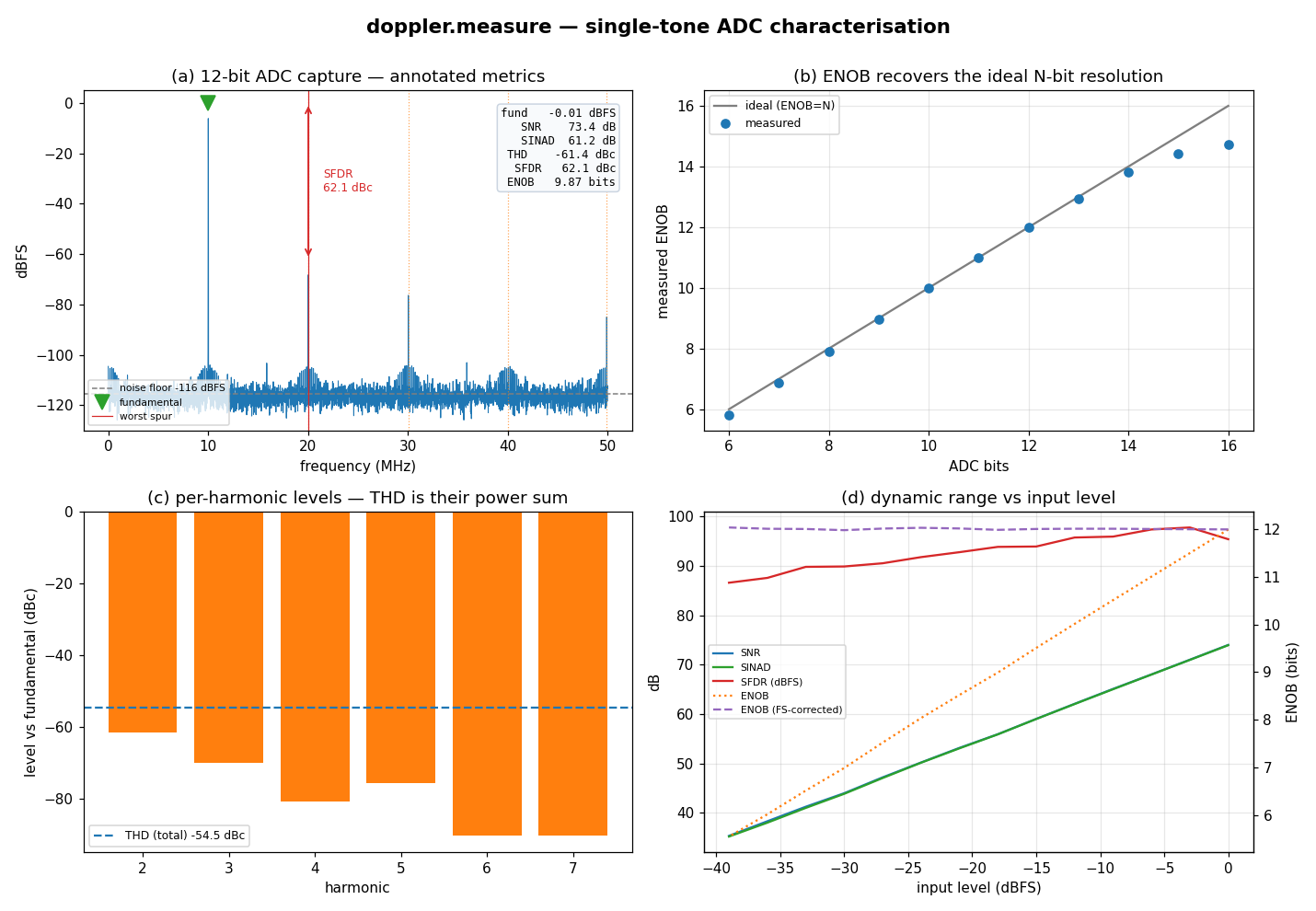
Panel (a) analyses a 12-bit ADC capture: the fundamental reads 0 dBFS, the
~74 dB quantisation SNR is visible as the broadband floor, and SINAD/SFDR are
limited by the 2nd harmonic (the worst spur, flagged as harmonic). Panel (b)
sweeps ADC resolution and confirms the measured ENOB recovers the ideal N
for 6–16 bits. Panel (c) breaks out the per-harmonic levels that THD
aggregates. Panel (d) sweeps input back-off: SNR/SINAD/SFDR track the input,
while the full-scale-corrected ENOB stays flat — the converter's intrinsic
resolution, independent of how hard you drive it.