Detection Theory
Detection theory curves
doppler.detection implements the closed-form Marcum Q functions used
to set thresholds and predict detection probability without running
Monte Carlo. det_pd gives P_d for a given SNR and dwell;
det_dwell inverts it to find the minimum dwell that meets a P_d
target.
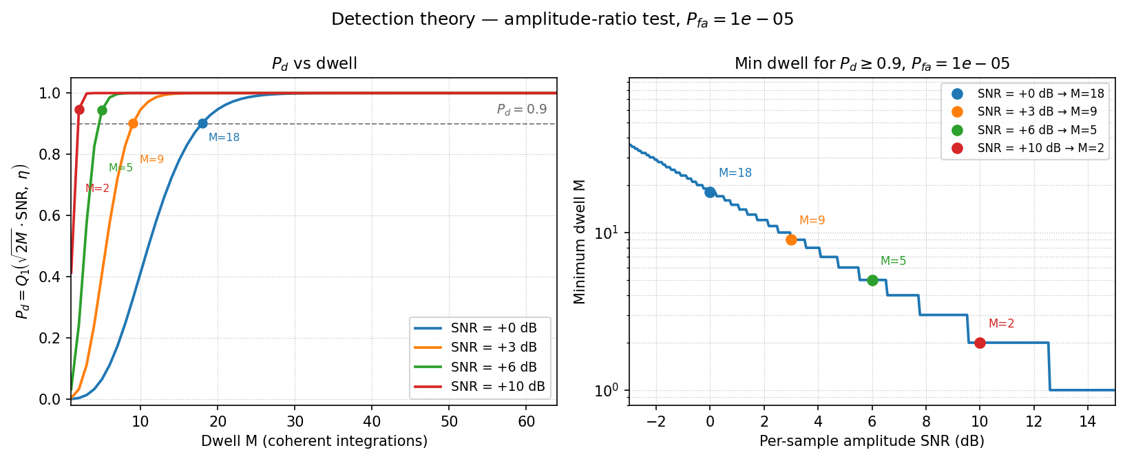
The right panel shows a key design insight: at P_fa = 1e-5 and P_d = 0.9, every 3 dB of extra SNR roughly halves the required dwell (coherent integration gain vs SNR).
from doppler.detection import det_pd, det_dwell, det_threshold
import numpy as np

PFA = 1e-5
eta = det_threshold(PFA)   # CFAR threshold parameter
print(f"eta = {eta:.4f}")

# Pd at 0 dB SNR after M coherent integrations
for M in [2, 5, 9, 18]:
    snr_amp = 1.0   # 0 dB amplitude SNR
    pd = det_pd(snr_amp, M, eta)
    print(f"dwell={M:2d}  Pd={pd:.3f}")

# Minimum dwell to reach Pd ≥ 0.9 at each SNR
for snr_db in [0, 3, 6, 10]:
    snr_amp = 10 ** (snr_db / 20)
    M = det_dwell(snr_amp, 0.9, PFA, 64)   # positional args
    print(f"SNR={snr_db:+d} dB  →  min dwell M={M}")
eta = 4.7985
dwell= 2  Pd=0.004
dwell= 5  Pd=0.066
dwell= 9  Pd=0.328
dwell=18  Pd=0.902
SNR= +0 dB  →  min dwell M=18
SNR= +3 dB  →  min dwell M=9
SNR= +6 dB  →  min dwell M=5
SNR=+10 dB  →  min dwell M=2
Run the full plot:
Monte Carlo vs Marcum Q theory
detection_sim.py validates both the envelope detector and power
detector against Marcum Q predictions using 30 000 independent trials
per SNR point. The left column shows empirical survival functions
overlaid on the closed-form curves; the right column plots P_d vs SNR.
MC and theory agree to within statistical noise throughout.
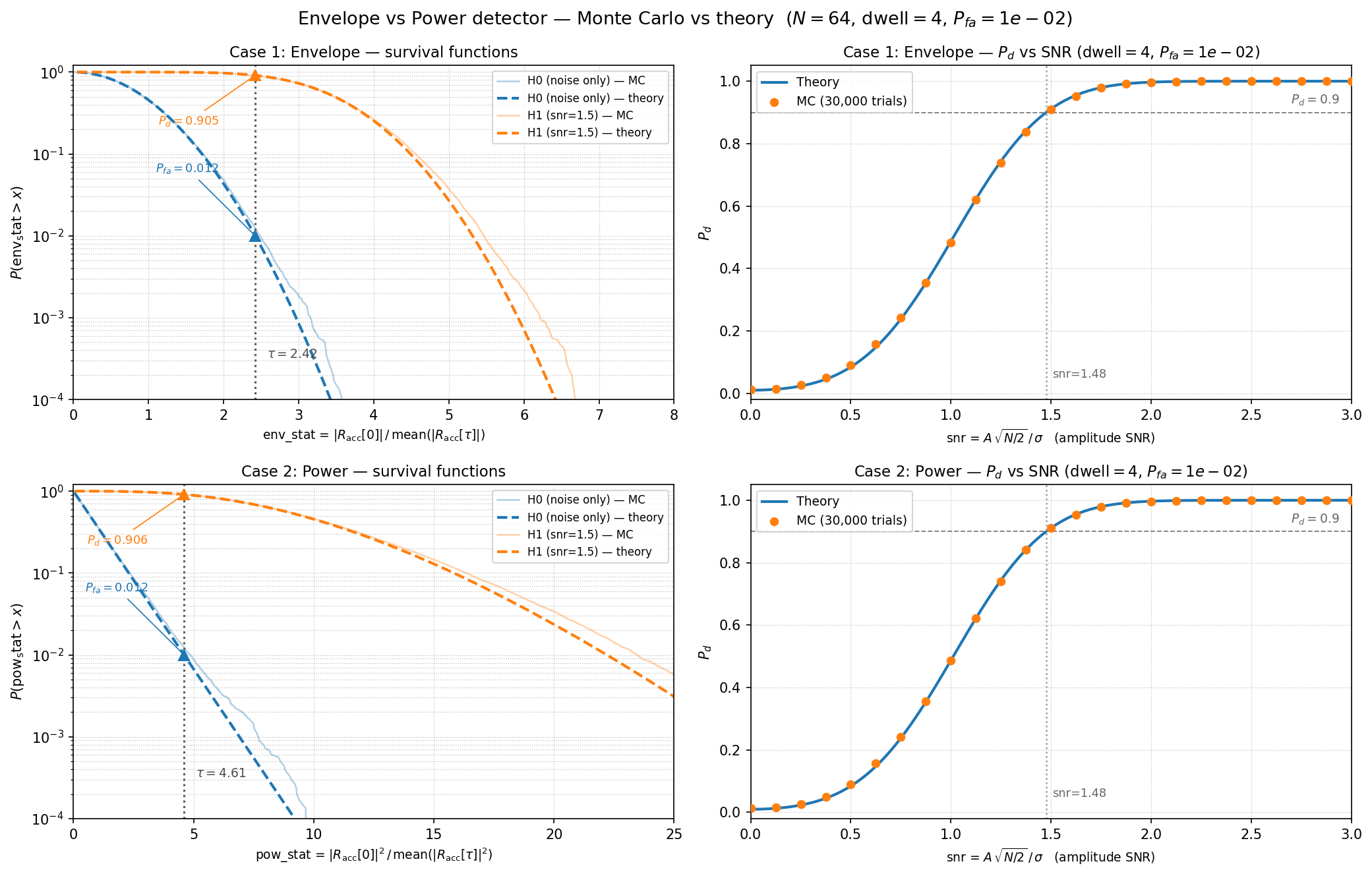
The simulation samples the matched-filter output directly from its theoretical distribution (Rician H1, Rayleigh H0) rather than running the full FFT pipeline, which avoids the degeneracy that appears when a single-bin tone is correlated against itself via FFT.