AGC Settling — a design chart¶
What you're seeing¶
How long to wait for an AGC to settle, as something you can read off rather than guess at.
agc_core.h gives the loop filter a time constant of 1/(4·loop_bw)
samples. The object is not the filter: the power detector sits inside
the loop and measures in power, so a quiet input's dB reading crawls up a
concave log. 1/(4·loop_bw) is therefore a floor, and anything derived
from it alone — a receiver's warm-up budget, say — is optimistic.
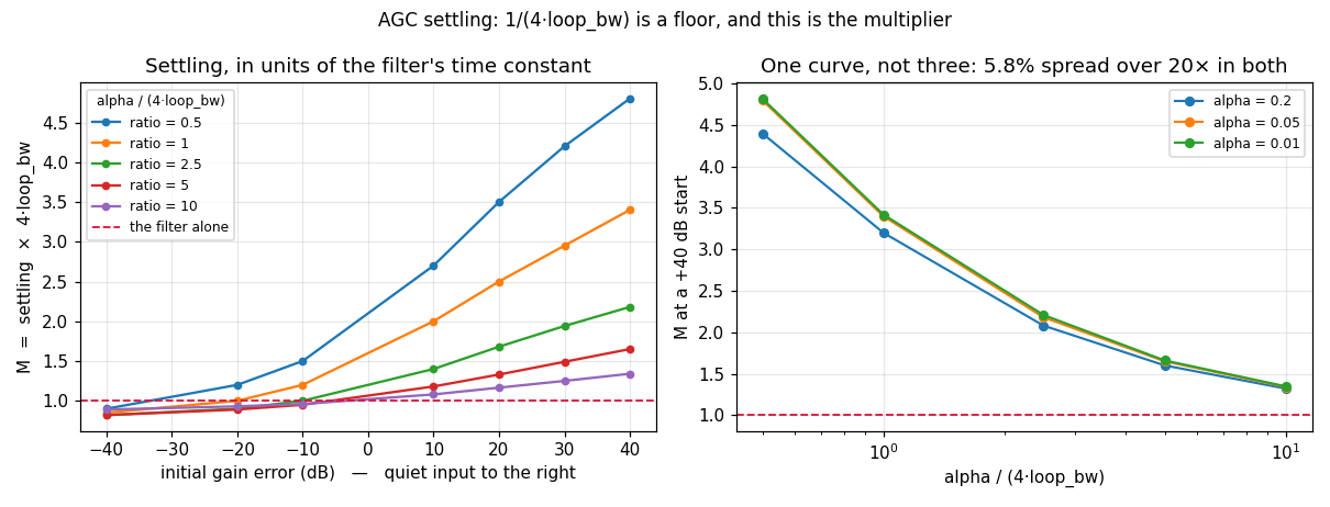
The left panel is the multiplier that turns the floor into an answer:
The crimson line at M = 1 is the filter alone. Every curve rises above it
to the right, because a quiet input is the slow case: at the widest
separation measured, a cold loop needing +40 dB of gain takes 4.8× what
its filter predicts.
Why the family is indexed by one number¶
M is not a free function of both alpha and loop_bw. It depends on the
initial gain error and on one dimensionless group — how fast the detector
is relative to the filter:
The right panel is that claim under test. Three alpha values spanning 20×,
each paired with the loop_bw that holds the ratio fixed, land on one
curve to within 5.8%. That is what makes the left panel a chart rather
than a table: measure it once, read it at any bandwidth.
The example asserts this rather than asserting it in prose — if the spread exceeds 10% the script fails, because at that point the chart cannot be read at an arbitrary bandwidth and should not be published as if it could.
Using it¶
- Pick
loop_bwfrom the disturbance you must track, andalphafrom how hard the envelope needs smoothing. Formratio = alpha / (4·loop_bw). - Take the largest gain error you expect to start from. For a cold receiver that is the whole input dynamic range it must cover, not the steady-state variation.
- Read
Moff the left panel and multiply by1/(4·loop_bw).
Worked, for the shipped MPSK_RX_AGC_ALPHA = 0.01 at bn_agc = 5e-4:
ratio = 0.01/(4·5e-4) = 5, so a +40 dB cold start costs M = 1.65 — about
1.65/(4·5e-4) ≈ 825 samples, against the 500 the filter alone would
suggest.
The script closes by predicting a configuration that built none of the
curves — loop_bw = 0.004, alpha = 0.02, a +25 dB start — and checking the
measurement against it. Predicted M = 2.73, measured 2.48, 9% out. A
design guide that has never been used to predict anything is a picture.
The direction nobody budgets for¶
The −40 dB column sits slightly below the floor: a loud input settles
marginally faster than the filter predicts, because the detector's EMA
climbs quickly in dB while the power is rising. It is real, it is small, and
it is the wrong direction to plan around — which is why the chart is drawn
with the quiet end on the right.
import math

import numpy as np

from doppler.agc import AGC

DIR = complex(0.6, 0.8)  # |DIR| == 1, so scaling exercises both components


def settle_multiplier(
    loop_bw: float, alpha: float, gain_err_db: float
) -> float:
    """1/e settling, in units of the filter's own time constant.

    The target is analytic — a constant input needing `gain_err_db` of gain
    converges there — so this measures against an external truth rather than
    against wherever the loop happens to stop, which would beg the question.
    """
    amp = 10.0 ** (-gain_err_db / 20.0)
    agc = AGC(ref_db=0.0, loop_bw=loop_bw, alpha=alpha)
    err0 = abs(gain_err_db)
    budget = int(40.0 / loop_bw)
    for n in range(budget):
        agc.step(DIR * amp)
        if abs(agc.gain_db - gain_err_db) <= err0 / math.e:
            return (n + 1) * 4.0 * loop_bw
    return float("nan")


# The design axes: how far the loop starts from home, and how fast the
# detector is relative to the filter.
ERRORS_DB = np.array([-40.0, -20.0, -10.0, 10.0, 20.0, 30.0, 40.0])
RATIOS = np.array([0.5, 1.0, 2.5, 5.0, 10.0])
ALPHA = 0.05

chart = np.array(
    [
        [
            settle_multiplier(ALPHA / (4.0 * r), ALPHA, float(e))
            for e in ERRORS_DB
        ]
        for r in RATIOS
    ]
)

# The reusability claim: same ratio, different (alpha, loop_bw), same M.
CHECK_ALPHAS = [0.2, 0.05, 0.01]
collapse = np.array(
    [
        [settle_multiplier(a / (4.0 * r), a, 40.0) for r in RATIOS]
        for a in CHECK_ALPHAS
    ]
)
Related¶
- AGC design — §2.2 for why the detector stays in the power domain, and §6 for the header claim this measurement corrected
- AGC validation report — §2.1 measures the same asymmetry as a certified limit
- Python AGC API