Ddcr — Real Passband to Baseband
What you're seeing
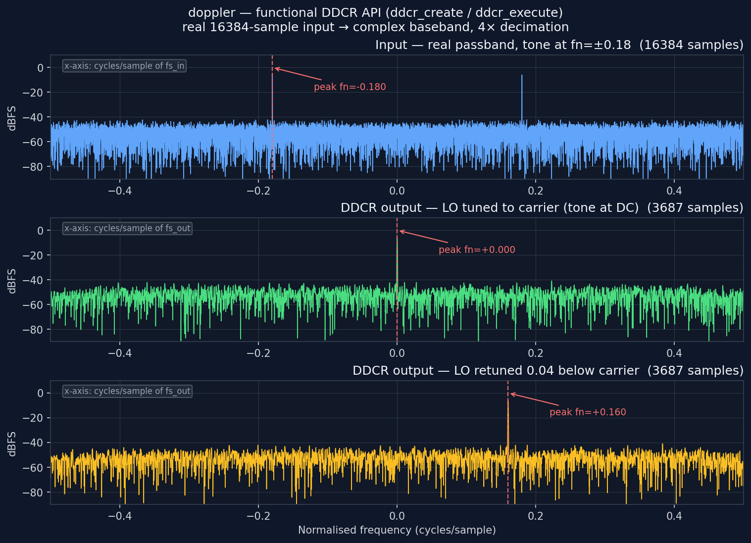
Three panels share the same x-axis — normalised frequency in cycles/sample (−0.5 to +0.5). A red dashed marker labels the strongest spectral line in each panel.
Top panel — input. 16384 samples of a real float32 signal: a tone at
fn = 0.18 (relative to the input sample rate fs_in) plus broadband noise.
Because the input is real, the spectrum is symmetric — the tone shows at both
±0.18.
Middle panel — baseband output. The same signal run through Ddcr.execute
with the NCO tuned so the carrier lands at DC. The output is complex64
and decimated 4× (rate = 0.25), so its x-axis is normalised to fs_out. The
tone sits at fn = 0.000.
Bottom panel — retuned output. The LO is moved 0.04 (in fs_in) below the
carrier via the norm_freq property. The tone shifts off DC by
0.04 / rate = 0.16 in fs_out units, landing at fn = +0.160 — exactly as
predicted, and phase-continuously (no filter-history reset).
One object over opaque C state
Ddcr is a generated class: a typed Python object over an
opaque ddcr_state_t *. It unifies what were once two faces (a DDCR object
and ddcr_* free functions) into one — it owns the C state like an object,
yet execute() writes into a caller-provided output buffer like the old
functional API, so allocation and lifetime stay explicit.
| Aspect | Ddcr |
|---|---|
| State | opaque ddcr_state_t *, owned by the object (RAII close) |
| Output | written into a caller-owned complex64 buffer |
| Retune | ddcr.norm_freq = … (live, phase-continuous) |
| Use when | real-ADC input; you manage your own arrays / want zero |
| per-call allocation in a hot loop |
How it works
A Ddcr takes a real passband signal, mixes it with a fine NCO (running at
fs_in / 2), low-pass filters, and decimates to complex baseband. To park
a real tone at carrier f_carrier (normalised to fs_in) at DC:
The lifecycle is explicit — the object is yours to keep, reuse, and release:
import numpy as np
from doppler.ddc import Ddcr

stream = [np.zeros(4096, dtype=np.float32) for _ in range(3)]  # demo blocks

ddcr = Ddcr(norm_freq=-(2 * 0.18 + 0.5), rate=0.25)

out = np.empty(4096, dtype=np.complex64)        # reused every block
for block in stream:                            # block: ndarray[float32]
    y = ddcr.execute(block, out)                # zero-copy view out[:n_out]
    ...

ddcr.norm_freq = -(2 * 0.14 + 0.5)              # retune, phase-continuous
ddcr.reset()                                    # zero all history
ddcr.close()                                    # release C resources
After close(), any further call raises RuntimeError; live
views of earlier output stay valid because they reference the caller's buffer,
not the state. A with Ddcr(...) as ddcr: block closes it automatically.
Streaming semantics — the object wraps mutable C state
A Ddcr wraps a single C pointer to a struct that is mutated in place on
every call. The actual state (the LO phase, the halfband taps, the polyphase
resampler banks, the history buffers) lives entirely in C and never crosses
the Python/C boundary: each call passes the object, not the kilobytes of
state, so nothing is serialized, marshaled, or copied per call. That is also
what makes block-by-block processing phase-continuous — the same object
carries its history forward from one execute to the next, so feeding a signal
as two halves through the same object is bit-identical to processing it in one
shot:
lo = -(2 * 0.18 + 0.5)                          # tune carrier fn=0.18 to DC
x = np.cos(2 * np.pi * 0.18 * np.arange(8192)).astype(np.float32)
out = np.empty(8192, dtype=np.complex64)

# one shot ----------------------------------------------------------------
d = Ddcr(lo, 0.25)
y_whole = d.execute(x, out).copy()

# same input, same handle, two blocks -------------------------------------
d = Ddcr(lo, 0.25)
y0 = d.execute(x[:4096], out).copy()   # state advances in place
y1 = d.execute(x[4096:], out).copy()   # picks up exactly where y0 left off
# np.concatenate([y0, y1]) == y_whole   (max|Δ| == 0)
Run those same two halves through fresh handles instead and the seam shows a
phase jump and a filter transient (max|Δ| ≈ 0.78) — the carried history is
exactly the in-place state. Setting norm_freq and calling reset() likewise
mutate the same handle.
Consequences:
- One handle = one stream. Don't share a handle across threads concurrently; give each stream its own.
- Deterministic lifetime.
close()frees the C resources when you say so, not when the GC happens to run. - The only value handed back is the output view (
out[:n_out]); everything else lives in — and mutates — the handle.
Performance — zero-copy, zero steady-state allocation
The handle is the same C core as the DDC object; on a 4096-sample block
all paths land within ~2 % (≈16 µs/block on this machine). The benefit is
where the output goes and what gets allocated, not raw throughput:
| Path | per-call allocation | output lands in |
|---|---|---|
ddcr.execute(x, out), out reused |
none (steady state) | a buffer you own |
ddcr.execute(x, np.empty(...)) |
one output array | a fresh array each call |
So the caller-buffer model buys you:
- Zero-copy into caller memory. Write results straight into a slice of a larger array, a memory-mapped region, or the next pipeline stage's input buffer — no copy to move the result into place afterward.
- Multiple live outputs. Target a different
outper call, so several outputs stay valid at once. - No per-call allocation in the steady state when you reuse one
out— small here (the allocator recycles the 32 KiB block cheaply), but it removes allocator traffic and GC pressure entirely, which matters under many parallel streams or tight real-time budgets.
Parallelism — execute releases the GIL
The C kernel runs with the GIL released (Py_BEGIN_ALLOW_THREADS around the
ddcr_execute call). It's safe precisely because of the one-handle-per-stream
contract: the kernel touches only that stream's state and the caller's
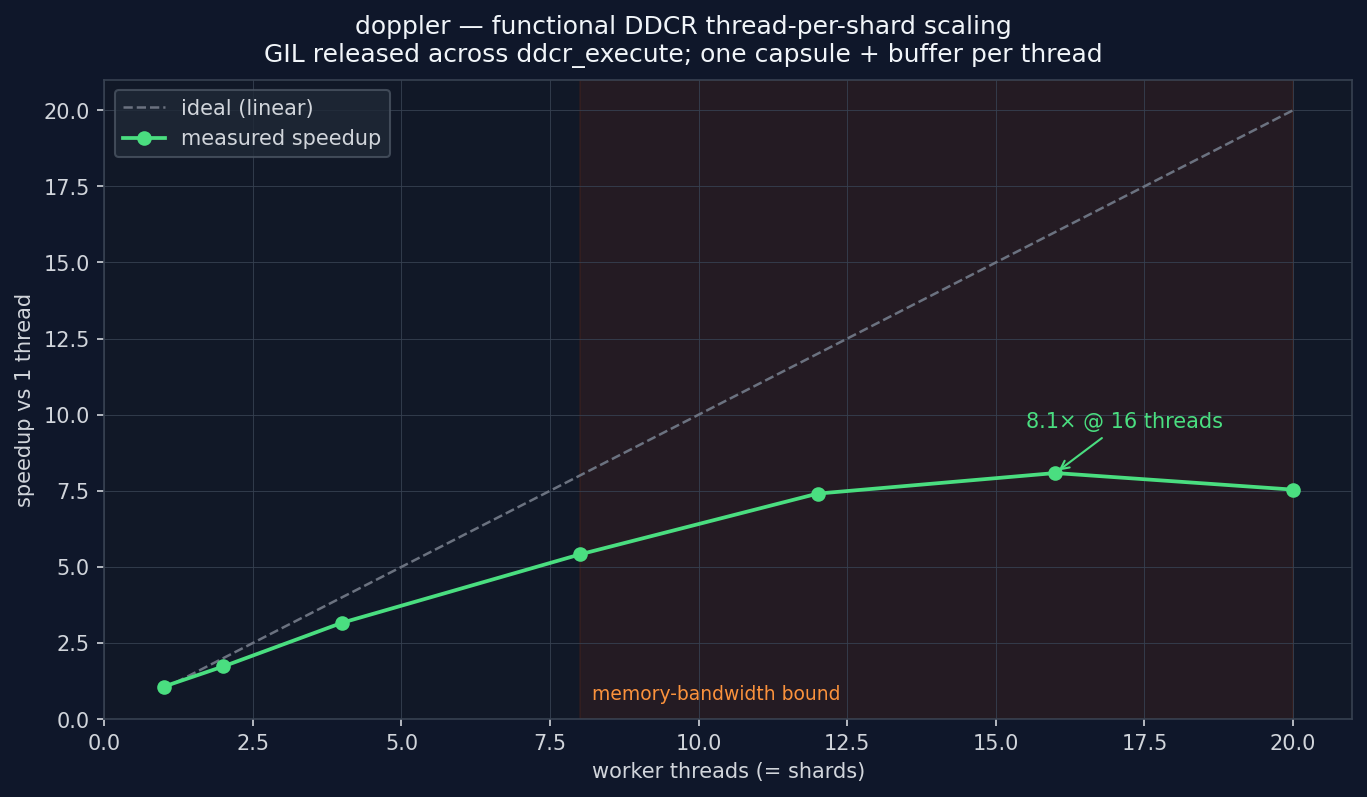
buffers — no Python objects, no shared mutable state. So a thread-per-shard
worker — each thread owning its own handle and out buffer — scales across
cores instead of serialising on the GIL:
| threads | speedup | efficiency |
|---|---|---|
| 1 | 1.00× | 100 % |
| 2 | 1.73× | 86 % |
| 4 | 3.16× | 79 % |
| 8 | 5.41× | 68 % |
| 12 | 7.41× | 62 % |
| 16 | 8.08× | 51 % |
(8192-sample blocks, representative run on a 20-core box; regenerate with
make gallery. Before releasing the GIL the same test was flat at ~1×
regardless of thread count.) Scaling is near-linear through a handful of cores
and then memory-bandwidth bound — the kernel streams large buffers, so past
~8–12 threads more cores stop helping. The takeaway for sizing: one replica can
use several cores via threads before you reach for process-per-shard, which
changes your replica-count math.
This pairs directly with the streaming model above: shard by stream, give each worker thread a disjoint set of handles, and there is no shared state to lock — the parallelism is embarrassingly so.
In short: same speed, but you own the buffer and the lifetime — exactly what a zero-copy streaming pipeline wants.