AGC — Step Response
What you're seeing
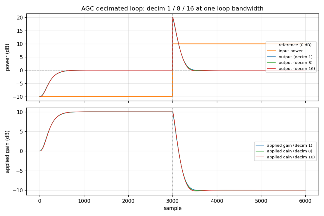
A 6000-sample complex tone that steps from −10 dBm to +10 dBm at sample
3000. Three curves overlay almost perfectly because all three use the
same loop_bw = 0.00125; only the decimation factor changes how often
the loop ticks.
- decim=1 — loop updates every sample; fastest per-sample cost.
- decim=8 — loop updates every 8 samples; ×8 cheaper, identical trajectory.
- decim=32 — coarsest timing; still converges within ~350 samples of the 20 dB step.
The gain trace is output power in dBFS. All three curves converge to 0 dBFS before the step and recover to 0 dBFS within ~350 samples after it.
How it works
agc_steps() rescales the loop coefficients by decim so that
loop_bw keeps its per-sample meaning regardless of how coarsely
the detector ticks.
from doppler.agc import AGC
import numpy as np

n = np.arange(6000)
amp = np.where(n < 3000, 10**(-10/20), 10**(10/20))
x = (amp * np.exp(2j * np.pi * 0.02 * n)).astype(np.complex64)

agc = AGC(ref_db=0.0, loop_bw=0.00125, alpha=0.02)
agc.decim = 8          # update loop every 8 samples
y = agc.steps(x)       # normalised output, power → 0 dBm
alpha controls the exponential moving-average window for the power
detector; loop_bw sets the first-order loop bandwidth. Wider
loop_bw → faster tracking but more noise at steady state.
See AGC API walkthrough for the full parameter reference and decimated-loop derivation.