wfmgen — One Engine, Every Waveform¶

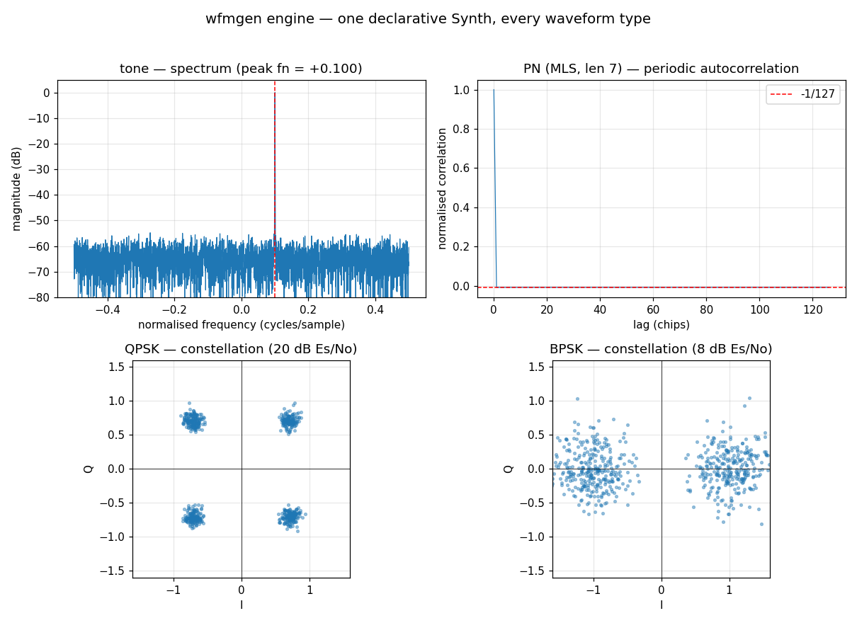
What you're seeing¶

A single declarative engine — doppler.wfm.Synth, the same C core the wfmgen command-line tool run — produces every waveform type, shown here through the view that makes each one's structure obvious.

Top-left — tone. A complex baseband tone at fn = 0.10 (relative to fs) at 30 dB SNR over the sample rate. Because the signal is complex, the spectrum has a single line at +0.10 with no mirror image; the red marker labels the peak.

Top-right — PN. A maximum-length sequence (LFSR register length 7 → period 127) at one chip per sample. Its periodic autocorrelation is the MLS "thumbtack": 1.0 at zero lag and a flat −1/127 floor at every other lag — the property that makes an MLS a good spreading and ranging code. --pn_poly 0 selects the primitive polynomial for the chosen length automatically.

Bottom-left — QPSK at 20 dB Es/No and bottom-right — BPSK at 8 dB Es/No, both after a boxcar matched filter over each symbol (the receiver view that realises the Es/No — integrating a symbol's sps samples buys 10·log10(sps) dB over a single mid-symbol sample). QPSK's four Gray-coded points and BPSK's two antipodal points sit exactly where the modulation places them; the cloud size is the symbol-energy SNR made visible.

The engine and its CLI¶

Every type, SNR mode, and the MLS auto-polynomial live once in C (native/src/wfm_synth/wfm_synth_core.c, generated from objects/wfm_synth.toml), and one command-line tool — wfmgen — exposes it:

`wfmgen`
Scope	one waveform from flags, or a multi-segment scene
Spec	flags or `--from-file spec.json`
Containers	`raw`, `csv`, BLUE-1000, SigMF
Output	file / stdout / `zmq://`
Provenance	`--record run.json` (replays byte-identically)

The same engine is the doppler.wfm Python API; a one-segment wfmgen run is the simple single-waveform case of the composer.

Smart defaults¶

The goal is that a bare command Just Works and you only dial in what you need:

wfmgen --type tone                  # clean baseband tone, fs 1 MHz, 1024 cf32
wfmgen --type qpsk --snr 12         # QPSK at 12 dB Es/No (the auto mode for *psk)
wfmgen --type pn --pn_length 9      # length-9 MLS, primitive poly chosen for you

--snr_mode auto resolves per type: over-fs for tone/noise/pn, Es/No for bpsk/qpsk. Override with --snr_mode fs|ebno|esno.
--snr 100 (the default) is effectively clean — raise the noise by lowering it.
--pn_poly 0 picks the maximum-length polynomial for --pn_length.

Containers, sample types, byte order¶

The sample type (--sample_type cf32|cf64|ci32|ci16|ci8, full-scale ±1.0 for the integer types) is orthogonal to the container and byte order:

# 16-bit I/Q, big-endian, into a self-describing BLUE type-1000 file
wfmgen --type qpsk --count 100000 --sample_type ci16 --endian be \
       --file_type blue -o capture.blue

# SigMF pair: capture.sigmf-data (raw) + capture.sigmf-meta (one annotation
# per segment, with frequency edges and the waveform label)
wfmgen --from-file scenario.json --sample_type ci16 --file_type sigmf -o capture

# stream to a ZMQ PUB endpoint a doppler subscriber can read
wfmgen --type tone --continuous --output zmq://tcp://*:5555

BLUE carries fs (as xdelta = 1/fs), the complex sample format, and byte order in its 512-byte header, so one file is fully self-describing.

Multi-segment specs and reproducible runs¶

--record FILE writes the fully-resolved spec as JSON — every value after defaulting (the chosen MLS polynomial, the resolved SNR mode, …). Feed that file straight back with --from-file and you get a byte-identical stream:

wfmgen --type bpsk --count 50000 --sps 4 --record run.json -o a.iq
wfmgen --from-file run.json -o b.iq      # a.iq and b.iq are identical

A multi-segment spec sequences waveforms with off-time gaps, and can repeat or run forever:

{
  "version": "wfmgen-1", "repeat": false, "continuous": false,
  "segments": [
    { "type": "tone", "fs": 1e6, "freq": 1e5, "snr": 100.0,
      "num_samples": 10000, "off_samples": 5000 },
    { "type": "qpsk", "fs": 1e6, "snr": 9.0, "snr_mode": "esno",
      "sps": 8, "num_samples": 40000, "off_samples": 0 }
  ]
}

PN codes — length, polynomial, realization¶

The PN/LFSR register runs from 2 to 64 bits; --pn_poly 0 (the default) auto-selects a verified primitive polynomial for the length, so every auto code is a true maximum-length sequence. --lfsr picks the realization — galois (default, internal XOR) or fibonacci (external XOR) — same polynomial and period 2ⁿ−1, different chip ordering.

wfmgen --type pn --pn_length 23 --sps 1                 # length-23 MLS (auto poly)
wfmgen --type pn --pn_length 40 --sps 1                 # 64-bit register, auto MLS
wfmgen --type pn --pn_length 9  --sps 1 --lfsr fibonacci

import numpy as np
from doppler.wfm import PN

# Galois and Fibonacci realizations of the same length-9 polynomial:
# identical period (511) and balance, different ordering.
galois    = np.asarray(PN(0x108, 1, 9, lfsr="galois").generate(511))
fibonacci = np.asarray(PN(0x108, 1, 9, lfsr="fibonacci").generate(511))
assert galois.sum() == fibonacci.sum() == 256      # 2**8 ones, balanced
assert not np.array_equal(galois, fibonacci)        # distinct sequence

A multi-segment spec can carry "lfsr": "fibonacci" and a 64-bit "pn_poly" per segment.

Detached BLUE headers¶

--detached (BLUE only) splits the container into a header + data pair — <out>.hdr (the 512-byte HCB, with detached=1 / data_start=0) and <out>.det (the raw samples). Attached output keeps whatever extension you give -o (.blue / .prm / …).

wfmgen --type qpsk --sps 8 --count 50000 \
       --sample_type ci16 --file_type blue --detached -o capture
# → capture.hdr (512-byte HCB) + capture.det (raw interleaved I/Q)

Reproduce¶

python examples/python/wfmgen_demo.py    # the four-waveform figure (writes .png)
python examples/python/pn_codes.py       # PN MLS / Galois vs Fibonacci / 64-bit

From Python — the composer API¶

The same composer is available in Python (doppler.wfm), producing byte-identical output to the CLI:

from doppler.wfm import Composer, Segment, Writer

spec = [Segment("pn", num_samples=127), Segment("qpsk", num_samples=4096,
                                                off_samples=512)]
with Writer("frame.cf32", sample_type="cf32") as w:
    w.write(Composer(spec).compose())

See the Python composer API for Writer containers (raw / CSV / BLUE / SigMF), the ZmqSink, JSON round-tripping, and the rrc_taps / dsss_spread / mls_poly helpers.