AWGN Generator

What you're seeing

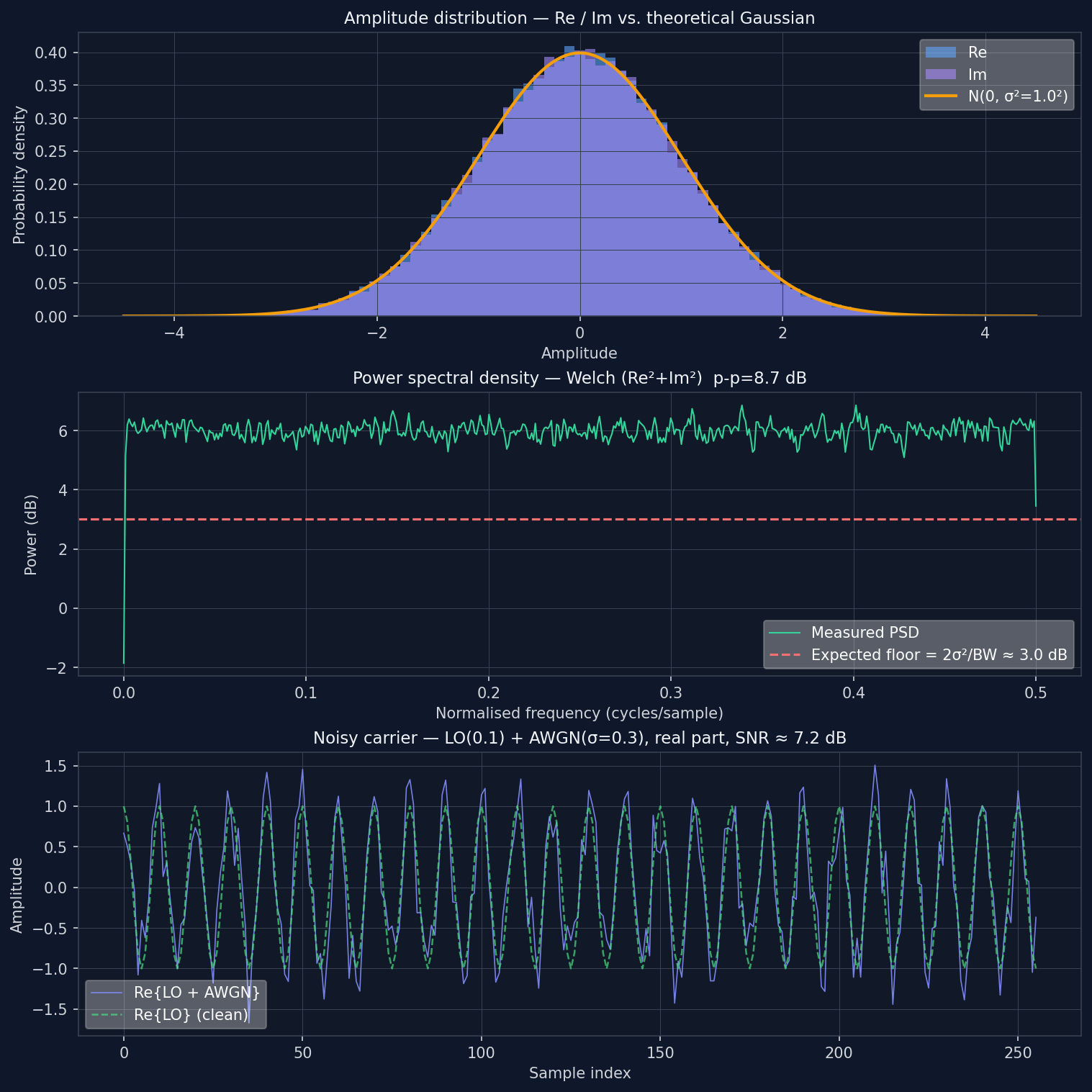
Top panel — amplitude histogram. Real and imaginary components of 65 536 CF32 samples with amplitude=1.0 overlaid with the theoretical N(0, σ²=1) Gaussian PDF. Both components track the curve to within statistical noise, confirming the Box-Muller transform is unbiased.

Middle panel — Welch PSD. One-sided power spectral density of 65 536 samples (Re²+Im², nperseg=1024). The trace stays within ±1 dB of the expected floor across the full bandwidth, confirming the spectrum is white — no tonal artefacts from the LUT phase quantisation.

Bottom panel — noisy carrier. Real part of LO(0.1) + AWGN(σ=0.3), first 256 samples. The clean carrier (dashed) rides underneath the noise. Total complex power is split evenly: carrier ≈ 1/√2 per component, noise σ=0.3 per component, giving ≈ 10 dB SNR.

How it works

from doppler.source import AWGN

g = AWGN(seed=42, amplitude=1.0)
noise = g.generate(65536)   # complex64 array

Each complex output sample consumes two 64-bit xoshiro256++ words:

u1 = (top-24-bits(word0) + 1) × 2⁻²⁴  ∈ (0, 1]   — Box-Muller uniform
idx = top-16-bits(word1)                           — 65 536-entry LUT index
r   = amplitude × sqrt(−2 × ln u1)                — Box-Muller radius
out = r × cos(idx) + j × r × sin(idx)             — complex Gaussian

amplitude is the per-component standard deviation. Total complex power = 2 × amplitude².

The AVX-512 path runs 8 independent xoshiro256++ streams in parallel, uses glibc libmvec _ZGVdN8v_logf for 8-wide vectorised log, and reads sin/cos from the same 65 536-entry LUT as LO via AVX gather instructions — reaching ~525 MSa/s on a single AVX-512 core.

python examples/python/awgn_demo.py   # → docs/assets/awgn_demo.png

C one-shot (no persistent state):

float complex out[1024];
awgn(0, 1.0f, 1024, out);   /* seed=0, amplitude=1.0; returns 0 on success */

C stateful (streaming / replay):

awgn_state_t *g = awgn_create(42, 1.0f);
awgn_generate(g, 1024, out);
awgn_destroy(g);

See doppler.source.AWGN for the Python API reference, and examples/c for the full C examples.