A Crowded Band — Many Signals, One Parallel prepare¶

Composing a waveform gets expensive exactly when a single segment carries many signals — a fully-loaded band of carriers, a multi-user CDMA cell, a dense interference scene. Each signal is its own DSP (modulation, root-raised- cosine pulse shaping, a mix to its channel centre), and none of them depend on the others: the segment is just their sum. That independence is the opening. prepare renders each source once into its own cache buffer, and — because those builds share nothing — fans them across the machine's cores. The sum is deferred to render time, so the cached result stays bit-for-bit identical to a full serial compose; only the wall-clock changed.

What you're seeing¶

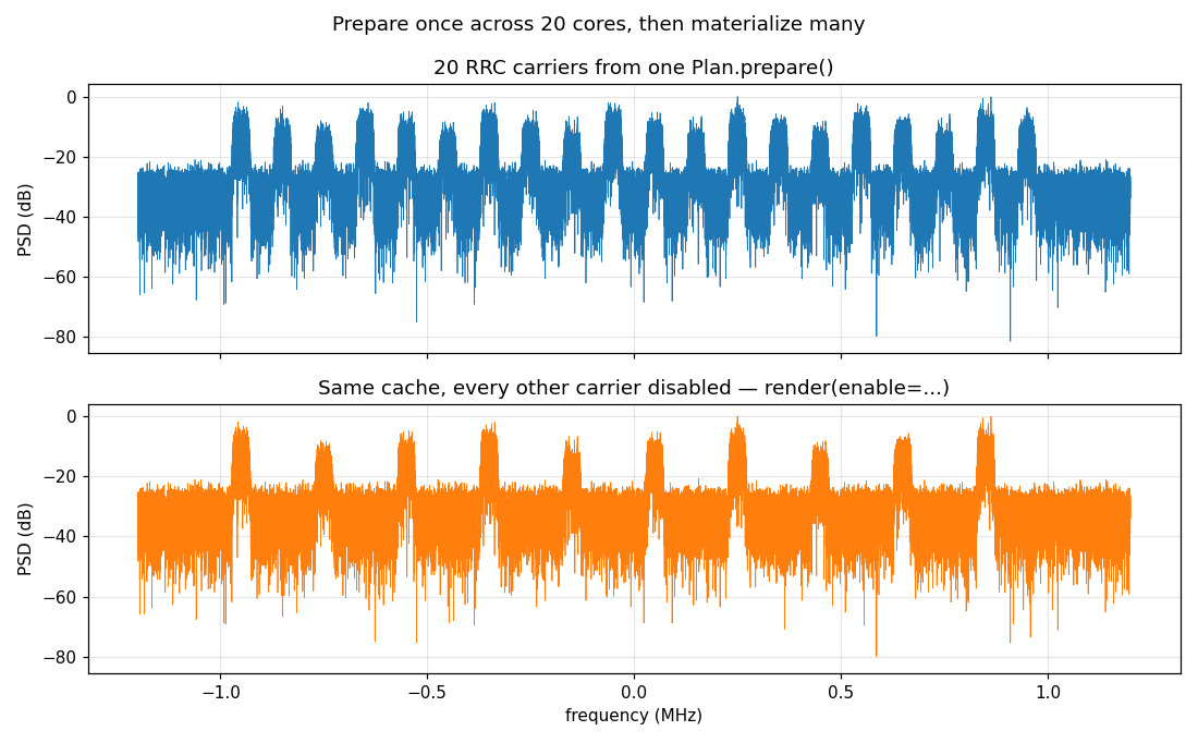
The scene is twenty RRC-shaped QPSK carriers spaced across a 2.4 MHz span, at three power tiers, over the AWGN floor implied by the anchor carrier. One Plan drives the whole figure.

Top — the crowded band. Every one of the twenty carriers, rendered from the prepared cache. This baseline is not an approximation: plan.render() is asserted equal, sample for sample, to Composer.compose() of the same scene.

Bottom — a variation for free. render(enable=...) disables every other carrier — an exact gain = 0 term applied to the same cache, with no re-synthesis. The odd carriers collapse into the noise floor while the survivors are untouched; the gaps open up at zero DSP cost. Sweeping levels, phases, the SNR, or the noise seed works the same way, which is what makes a Plan the right tool for a campaign that re-runs one scene hundreds of times.

How it works¶

Build the scene — twenty independent carriers summed into one segment:

import numpy as np

from doppler.wfm import Composer, Segment, prepare, qpsk

FS = 2.4e6  # occupied span (Hz)
N = 1 << 16  # 65,536 samples — well past prepare()'s parallel threshold
N_CARRIERS = 20  # a densely-loaded band: twenty signals in one segment
SPS = 64  # samples per symbol → ~37.5 kHz symbol rate, narrow carriers
SPACING = 100e3  # carrier spacing (Hz)
ANCHOR_SNR = 20.0  # carrier 0 carries the channel SNR; it sets the floor
_F0 = -(N_CARRIERS - 1) / 2.0 * SPACING  # first offset (band centred on DC)


def crowded_band() -> Composer:
    """Twenty RRC-shaped QPSK carriers over the AWGN floor set by carrier 0.

    Each carrier is fully independent DSP — QPSK symbols, a 2049-tap
    root-raised-cosine pulse (``2*rrc_span*sps + 1``), and a mix to its own
    channel centre — so ``prepare()`` fans the twenty per-carrier builds out
    across cores. Three power tiers (0 / -3 / -6 dBFS) keep it interesting.
    Carrier 0 carries the channel SNR (the resolver derives one shared noise
    floor from it); the rest are clean.
    """
    carriers = [
        qpsk(
            freq=_F0 + k * SPACING,
            snr=ANCHOR_SNR if k == 0 else 100.0,  # carrier 0 is the anchor
            seed=10 + k,
            sps=SPS,
            pulse="rrc",
            rrc_beta=0.25,
            rrc_span=16,
            level=-3.0 * (k % 3),
        )
        for k in range(N_CARRIERS)
    ]
    return Composer(Segment.sum(*carriers, fs=FS, num_samples=N))

Prepare it once, then materialize variations from the cache. prepare() is where the twenty per-carrier builds fan across cores; everything after is a re-weighted sum:

# prepare() renders every carrier ONCE and caches it — fanning the twenty
# independent per-carrier builds across cores — then render() serves each
# variation as a cheap re-weighted sum of that cache, never re-synthesising.
scene = crowded_band()
plan = prepare(scene)

# The cache is exact: a baseline render is bit-for-bit a full serial compose.
assert np.array_equal(plan.render(), scene.compose())

# Materialize a variation for free: disable every other carrier (the noise
# floor, handled separately, stays put). `enable` is per signal source.
_survive = [k % 2 == 0 for k in range(N_CARRIERS)]
thinned = np.asarray(plan.render(enable=_survive))

The parallelism is entirely inside prepare() — the public API does not change, and neither does a single output sample. The build is gated so that only a segment with more than one source and a long enough on-time crosses into the threaded path; small scenes stay serial and pay nothing for the machinery. On a 20-core machine this scene prepares in ~90 ms versus ~600 ms serially — the win grows with the number of signals and the sample count, since that is exactly the independent per-source work the fan-out spreads.

prepare, Plan, Composer, Segment and qpsk all come from doppler.wfm.

Reproduce¶

python -m doppler.examples.crowded_band_demo crowded_band_demo.png

Source: crowded_band_demo.py