Capturing All Receiver Telemetry
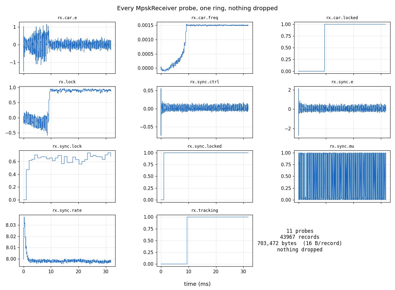
What you're seeing
Every panel is one telemetry probe a track.BpskReceiver exposes — except
the recovered symbol, where rx.sym.i and rx.sym.q share one axis because
the thing worth seeing is their relative size, and separate panels would
autoscale that away. Every trace came out of a single
telemetry.MemoryCapture over a
single telemetry.Telemetry ring. One set_telemetry attach registers
the receiver's own carrier probes and forwards to both of its
instrumented children — the symbol-timing loop and the front-end AGC — so a
cold-start BPSK pull-in leaves a complete record of the whole receiver:
rx.sym.i/rx.sym.q— the recovered symbol, and the only probe here that is an output rather than a loop internal. Sharing one axis is what makes it readable: I settles into two clean ±1 decision bands while Q collapses onto zero, which is the carrier loop resolving phase — a BPSK decision is real, so everything left in Q is error. The example asserts it (mean|I| ≈ 17× mean|Q| over the settled half), so the figure and the check are the same claim rather than two.rx.lock/rx.car.locked— the carrier lock EMA rises off its cold-start value andrx.car.lockeddeclares. The panel carries the declare and drop thresholds the decision actually used, read off the receiver (lock_thresh,lock_drop_thresh) rather than retyped here, so the line and the decision it drives cannot drift apart.rx.car.locked— the verify-counted decision on that statistic. It is an indicator and nothing more: there is no handover, so one M-th-power NDA discriminator steers the LO from the first output to the last (Mode 1 in the design), nothing waits for anything, and the transient is simply the cost of starting cold. Therx.trackingprobe that used to sit here was flat at 0 by construction — a probe that cannot vary is not a diagnostic — and it went with the handover in #877.rx.car.freq— the tracked NCO frequency pulls in to the injected 0.0015 cyc/sample offset.rx.car.e/rx.sync.e/rx.sync.ctrl— the carrier discriminator and the timing TED / loop-filter control settle out of the acquisition transient.rx.sync.rate/rx.sync.mu— the tracked samples/symbol settles on ~8.0 and the fractional interpolation phase sweeps its[0, 1)range.rx.sync.lock/rx.sync.locked— the timing lock statistic climbs and its verify-counted decision declares, against its own threshold (sync_lock_thresh), which is not the carrier's number and is not derived the same way — symsync sizes block length and threshold together from (rolloff, esno_min, pfa, pd). Declare and drop are the same level here and the panel says so in one line: the timing decision's hysteresis is in its verify counts, not its levels.rx.agc.gain_db/rx.agc.level_db— the front-end AGC, which bympsk_rx_agc_bn()is the slowest of the receiver's three loops. Here it has nothing to do: the stimulus is unit-magnitude symbols against a 0 dB reference, so the loop starts converged and both traces are dither —level_dbholding the reference inside a few tenths of a dB while the commanded gain wanders by hundredths. That is the point worth reading off this panel.level_dbis the loop's input, so "converged" is legible from the trace alone;gain_dbsettles to an offset that depends on how loud the input happened to be, and cannot be judged without knowing it. A cold, off-reference start is where the pair separates, and that measurement belongs with the AGC's own evidence rather than here.
Nothing is decimated (decim=1) and nothing is dropped — the summary cell
reports the full capture: 16 probes, one 16-byte record per event. For the
fourteen carrier, timing and symbol probes an event is a recovered symbol;
the two
rx.agc.* probes are tapped pre-terminal, ahead of the stage the timing
loop steers, and emit once per gain update instead, so they are denser and
carry no symbol index. The x-axis is real time, because each record carries
the sample index it was stamped with — which is what lets two probes counted
on different grids be read against each other at all.
How it works
Two things the caller no longer does. The drain: a MemoryCapture
sizes the ring from the probe count and the block, and set_now(i) drains
at every boundary — so losslessness is arithmetic rather than a cadence you
have to get right, and close() raises if a record was lost anyway.
The split: read_dict(index=True) returns {name: (n, values)}, so
nothing below filters by probe id, inverts an id-to-name map, or plots an
event ordinal in place of a time axis.
import tempfile
from pathlib import Path

import numpy as np

from doppler.telemetry import MemoryCapture, Telemetry
from doppler.track import BpskReceiver
from doppler.wfm import Composer, SampleClock, Segment

FS = 1e6  # sample rate, and therefore the figure's time axis
RS = 125e3  # symbol rate — 8 samples/symbol, but nothing here says "8"
BLOCK = 256  # the step of our own loop — and the capture's whole contract
BN_CARRIER = 0.02

# The carrier offset, seeded AT the loop's acquisition bound and not past it.
# The bound is `bn_carrier / m` cycles per SYMBOL (the m because the NDA
# discriminator is an M-th power), so it is stated in those units and
# converted to the cycles per sample the stimulus advances in exactly once.
# This demo used to seed 0.0015 cyc/sample against a QPSK bound of 0.005
# cyc/symbol — 2.4x outside it, where acquisition is a coin flip rather than
# a demonstration (doppler#843).
OFFSET_SYM = BN_CARRIER / 2  # cycles per symbol, at the bound
OFFSET = OFFSET_SYM * RS / FS  # cycles per sample, for the stimulus

# The stimulus is built by `wfmgen`'s composer, not by numpy. Source
# generation is C-first, and this is the same path the CLI and the JSON
# record drive -- so the demo exercises the shipped transmitter instead of a
# second one written to resemble it.
#
# What that replaces is worth naming, because each line was a copy of
# something the library already owns: `np.repeat` for a rectangular pulse,
# `exp(2j*pi*OFFSET*k)` for the carrier offset, and
# `sqrt(8 / (2 * 10**(20/10)))` for the noise level -- an Es/N0 conversion
# that is `snr_mode="esno"` here and `wfm_snr_over_fs()` in C. A demo that
# re-derives the transmitter cannot catch a transmitter bug.
NSYM = 4000
SPS = int(FS / RS)
iq = np.asarray(
    Composer(
        [
            Segment(
                type="pn",  # maximal-length payload; no numpy RNG
                pn_length=15,  # period 32767 >> NSYM, so it never repeats
                seed=1,
                modulation="bpsk",
                pulse="rect",  # NRZ, matching the I&D the receiver derives
                sps=SPS,
                snr=20.0,
                snr_mode="esno",  # 20 dB MATCHED Es/N0, by the library's law
                freq=OFFSET * FS,  # cycles/sample -> Hz, converted once
                fs=FS,
                num_samples=NSYM * SPS,
            )
        ]
    ).compose()
)

# ONE ring; attach the receiver at decim=1 = EVERY event on EVERY probe. The
# attach registers the receiver's own probes AND forwards to its child loops,
# so this is the full set of "all available telemetry". Probes must be
# attached BEFORE the capture opens: the ring is sized from the probe table.
tlm = Telemetry()
# Stated in the units a capture comes with: two rates, in Hz. `sps` is
# `FS / RS` and the receiver computes it; `m` is carried by the type. Neither
# appears here, and `m_out` is DERIVED rather than pinned — which is not
# cosmetic: this demo pinned `m_out=4` against the default I&D pulse, and
# that pairing is measured at 3.11 dB off the coherent bound where the
# derived 8 is 0.41 dB off. A parameter nobody needed was costing the demo
# most of its margin.
# There is no handover: one M-th-power NDA discriminator steers the LO from
# the first output to the last, which is Mode 1 in `docs/design/mpsk.md` --
# nothing here waits for anything, and the transient is simply the cost of
# starting cold. `acq_to_track` was retired in doppler#877 along with the
# second discriminator it selected.
rx = BpskReceiver(
    sample_rate_hz=FS,
    symbol_rate_hz=RS,
    bn_carrier=BN_CARRIER,
    bn_timing=0.01,
)
rx.set_telemetry(tlm, "rx", 1)

# The capture owns the drain. `set_now(i)` marks the boundary and drains the
# block just finished; no ring size to guess, no read()/concatenate loop, and
# no post-hoc assert standing in for a guarantee. Leaving the block finalizes
# and RAISES if a record was lost — so reaching the next line is itself the
# losslessness proof — but it does not free, so the capture is still readable.
with MemoryCapture(tlm, BLOCK, SampleClock(FS)) as cap:
    for i in range(0, iq.size, BLOCK):
        tlm.set_now(i)
        rx.steps(iq[i : i + BLOCK])

series = cap.read_dict(index=True)  # {name: (sample_index, values)}
recs = cap.records()  # the same data, still 16-byte wire records

# The 16-byte record layout IS the capture format: .tofile() writes exactly
# the TLM16 payload tlm_sink frames onto the wire.
store = Path(tempfile.mkdtemp()) / "mpsk_tlm.tlm16"
recs.tofile(store)

assert rx.lock_time >= 0  # it declared, and lock_time dates the first one
assert set(series) == set(tlm.probe_names)  # every probe came back by name
assert sum(v.size for _, v in series.values()) == len(recs)  # nothing lost
assert store.stat().st_size == recs.nbytes == 16 * len(recs)
assert np.array_equal(np.fromfile(store, dtype=recs.dtype), recs)

# A BPSK decision is REAL, so a locked carrier loop leaves essentially
# nothing in Q -- measured over the settled half, mean|I| is ~17x mean|Q|.
# That is the claim the shared I/Q panel exists to make visible, and it is
# asserted here rather than left to the eye.
settled = len(series["rx.sym.i"][1]) // 2
mean_i = np.abs(series["rx.sym.i"][1][settled:]).mean()
mean_q = np.abs(series["rx.sym.q"][1][settled:]).mean()
assert mean_i > 8 * mean_q, f"carrier unresolved: {mean_i=:.3f} {mean_q=:.3f}"
The 16-byte record layout is the capture format. records() returns
the exact C dp_tlm_rec_t as a structured array
(n:u8, value:f4, probe:u2, flags:u2), so .tofile() writes it with no
transformation and those bytes are byte-for-byte the TLM16 payload that
dp_tlm_sink frames onto the NATS wire. File storage and streaming fan-out
share one format — the capture above verifies the round-trip bit-exact.
The ring stays SPSC: producer (steps) and consumer (the capture's drain)
run on one thread together, which is exactly why the boundary drain is both
the fastest option and the provable one.
For a capture you never need back in-process, Capture(tlm, block, path, clock) writes those same bytes straight to disk plus a <path>-meta JSON
sidecar carrying the probe registry and time base — self-describing, so a
reader needs nothing from the process that wrote it. To take the same
records across processes live, publish them as TLM16 frames instead; see
Many Emitters, One Consumer.
Run it
python src/doppler/examples/mpsk_telemetry_capture_demo.py # → mpsk_telemetry_capture_demo.png (~2 s)
See the telemetry API for the probe tables
and record layout, M-PSK Receiver for the receiver
itself, and Lock Detection for the verify-counted decisions
the *.locked / rx.tracking traces come from.