Doppler Channel — a Doppler Profile Driven by a Cosine¶

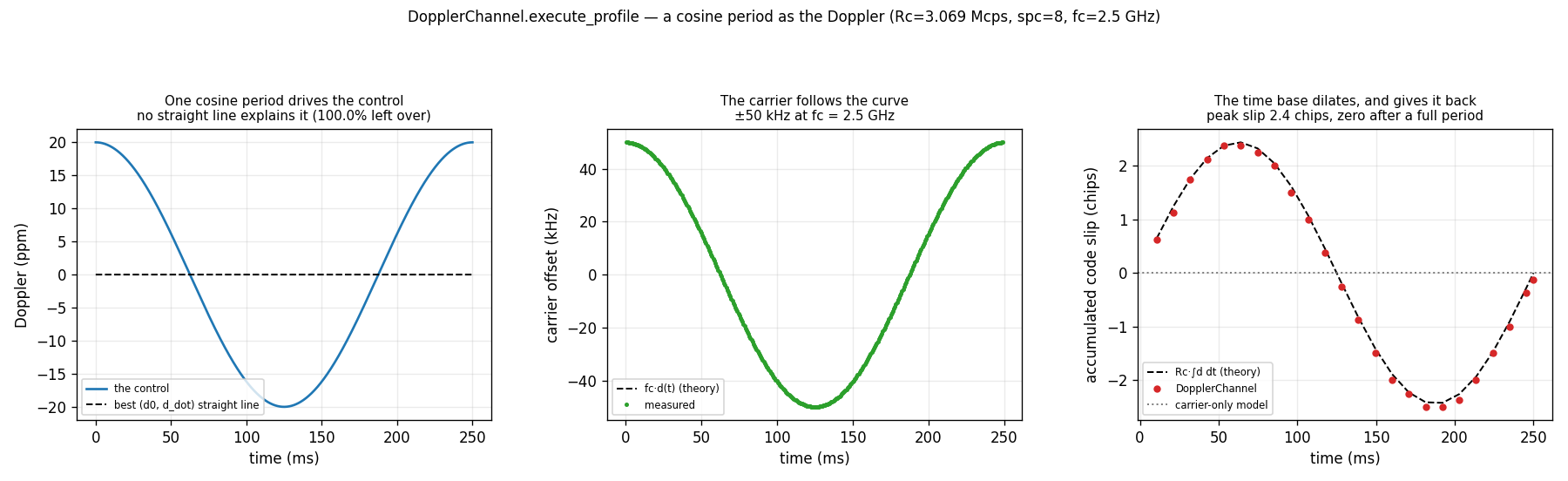
DopplerChannel takes its Doppler as a straight line, (doppler_ppm, doppler_rate_ppm_s). A real pass is not one: a satellite's range rate swings from closing to opening and back, so the Doppler it imposes is a curve. execute_profile(x, ppm) takes that curve as an array, one ppm value per input sample, and applies it.

Here the control is one full period of a cosine, d(t) = 20 ppm · cos(2π t / 0.25 s). It is the simplest curve no (d0, ḋ) can express, and it integrates in closed form, so everything the channel does is checked against an exact answer rather than against a second implementation.

What you're seeing¶

Left — the control. The cosine starts closing at +20 ppm, opens to −20 ppm and comes back. The dashed line is the best (d0, ḋ) straight line through the period: it is flat, and leaves 100.0% of the curve unexplained. This is the case the array form exists for.

Centre — the carrier follows the curve. At the 2.5 GHz carrier of the async DSSS receiver spec, 20 ppm is exactly ±50 kHz. The measured instantaneous offset sits on fc·d(t): the peak is 49 999.5 Hz against 50 000, and the worst difference over the whole period is 1.4 Hz (0.003% of the peak). What is left is the theory's argument: it is evaluated at the receive time, while the profile is indexed by the input (emission) clock, and the two differ by the excess delay, about 1e-5 relative.

Right — the time base dilates, and gives it back. This is the panel a carrier-only model gets wrong: it would be flat on the dotted line. The code slips by Rc·∫d dt = Rc·(A/ω)·sin(ωt), peaking a quarter of a period in at 2.44 chips in theory (2.50 as counted in whole samples) and returning to zero when the period ends, because the integral of a cosine over a whole period is zero. The trace is counted in whole samples (spc = 8), so an eighth of a chip is its floor. The same closure shows up in the stream's length: a full period is net-zero dilation, and the output is 6 138 001 samples for 6 138 000 in.

What the example asserts¶

The script is gated by make test-examples-python, so each of these is checked on every push, not just plotted:

• the stream fed in blocks is bit-identical to one call (the result must not depend on how it was chunked);
• the best straight line leaves more than 99% of the curve unexplained;
• the carrier offset is within 0.005% (2.5 Hz) of fc·d(t);
• the code slip follows Rc·∫d dt to within two samples (a quarter chip);
• the stream is within two samples of its input length.

How it works¶

The dilation is the resampler's per-sample rate control, fed one value per input sample. The carrier is not integrated beside it: the excess delay at output k is (p_k − k + 1)/fs, where p_k is the input position the resampler's own accumulator reports for that output. That is why the stream cannot depend on how it was chunked, and why the carrier cannot disagree with the dilation. The design page has the derivation, and the measurement record has the first attempt that mapped a profile index to an output index, and measured 2.75e-2 of chunk dependence.

import numpy as np

from doppler.impairment import DopplerChannel

CHIP_RATE = 3.069e6  # Mcps
SPC = 8  # samples per chip
FS = CHIP_RATE * SPC  # 24.552 MS/s
FC = 2.5e9  # RF carrier -- load-bearing, not metadata
AMP_PPM = 20.0  # +/-50 kHz at 2.5 GHz
PERIOD_S = 0.25  # one cosine period
N = round(FS * PERIOD_S)  # input samples in that one period
BLOCK = 1 << 18  # fed in blocks: the answer must not depend on this
BLOCK_B = 99_991  # a second, unrelated size: not a divisor of the first


def cosine_profile(n: int, amp_ppm: float) -> np.ndarray:
    """One full period of ``amp_ppm * cos`` over ``n`` input samples."""
    return amp_ppm * np.cos(2.0 * np.pi * np.arange(n) / n)


def drive(x: np.ndarray, ppm: np.ndarray, block: int = BLOCK):
    """Run ``x`` through the channel under ``ppm``, ``block`` at a time.

    The channel is created with no Doppler of its own: a profile is absolute,
    so the array is the whole story. Returns the output and, after each block,
    the (input, output) sample counts consumed so far.
    """
    ch = DopplerChannel(fs=FS, carrier_hz=FC)
    ys, counts = [], []
    n_in = n_out = 0
    for i in range(0, len(x), block):
        y = ch.execute_profile(x[i : i + block], ppm[i : i + block])
        ys.append(y)
        n_in += min(block, len(x) - i)
        n_out += len(y)
        counts.append((n_in, n_out))
    return np.concatenate(ys), np.array(counts)

Reproduce¶

python -m doppler.examples.doppler_channel_profile_demo doppler_channel_profile_demo.png

Source: src/doppler/examples/doppler_channel_profile_demo.py