A Streaming Spectrogram
A crowded band
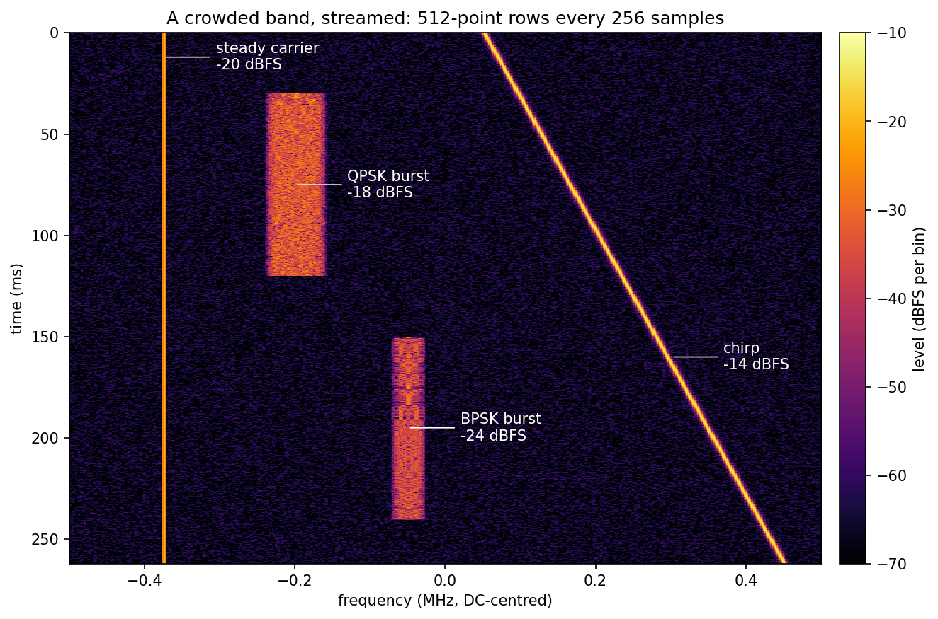
One capture, 262 ms at 1 MHz, streamed into 512-point rows every 256 samples and drawn in dBFS, time running down the page. Four signals share it: a steady carrier at −375 kHz, a chirp sweeping from +50 to +450 kHz, a QPSK burst that is on from 30 to 120 ms, and a BPSK burst from 150 to 240 ms. Under them is a noise floor of −40 dBFS in all, about −65 dBFS in each bin. The scene is built with the library's own waveform generator. Each burst is a segment of its own, silent outside its window and added to the steady part, so a burst starts and stops without disturbing anything around it:
SCENE_NFFT = 512  # 1953.125 Hz bins at FS = 1 MHz
SCENE_HOP = 256
SCENE_N = 1 << 18  # 262,144 samples: 262 ms
CARRIER_HZ = -375e3  # bin -192: on a bin centre, so it reads its own level
CARRIER_DB = -20.0
QPSK_HZ, QPSK_DB = -200e3, -18.0
BPSK_HZ, BPSK_DB = -50e3, -24.0
FLOOR_DB = -40.0  # the noise's total power, dBFS
QPSK_ON = (30e-3, 120e-3)  # seconds
BPSK_ON = (150e-3, 240e-3)


def burst(kind: str, freq: float, level: float, on: tuple, **kw) -> Segment:
    """One source, silent outside its on-window, as long as the scene."""
    start, stop = (int(t * FS) for t in on)
    return Segment(
        kind,
        fs=FS,
        freq=freq,
        level=level,
        delay_samples=start,
        num_samples=stop - start,
        off_samples=SCENE_N - stop,
        **kw,
    )


def crowded_band() -> np.ndarray:
    """A steady carrier, a slow chirp, two bursts, and the noise floor."""
    steady = Segment.sum(
        tone(freq=CARRIER_HZ, level=CARRIER_DB),
        chirp(freq=50e3, f_end=450e3, level=-14.0),  # sweeps the capture
        noise(level=FLOOR_DB, seed=1),
        fs=FS,
        num_samples=SCENE_N,
    )
    qpsk_burst = burst(
        "qpsk",
        QPSK_HZ,
        QPSK_DB,
        QPSK_ON,
        sps=16,
        pulse="rrc",
        rrc_beta=0.25,
        seed=7,
    )
    bpsk_burst = burst(
        "bpsk",
        BPSK_HZ,
        BPSK_DB,
        BPSK_ON,
        sps=32,
        pulse="rrc",
        rrc_beta=0.35,
        seed=11,
    )
    # Each part is composed on its own, so a burst can start and stop
    # without restarting the carrier, the chirp or the noise around it.
    parts = (steady, qpsk_burst, bpsk_burst)
    return sum(Composer(p).compose() for p in parts).astype(np.complex64)
The levels on the figure are measured, not just drawn. The script reads each level against the carrier. On its own bin the carrier reads −20 dB, and summed over its bins it is 10^(−20/10) times the window's noise bandwidth, so dividing a burst's summed bins by the carrier's cancels the window. Each burst then reads its own level inside its window and nothing outside it, the empty band reads the floor spread over 512 bins, and the strongest bin in the upper half follows the chirp's sweep to within one bin:
def band_power(power: np.ndarray, f_hz: float, half_bins: int) -> np.ndarray:
    """Per row, the sum of the linear bins within half_bins of f_hz."""
    c = SCENE_NFFT // 2 + round(f_hz / (FS / SCENE_NFFT))
    return power[:, c - half_bins : c + half_bins + 1].sum(axis=1)


def make_scene_figure(out_path: str = "spectrogram_scene.png") -> None:
    """Draw the crowded band as a dB waterfall, after checking it."""
    x = crowded_band()
    power = stream_rows(x, "power", SCENE_NFFT, SCENE_HOP)
    db = stream_rows(x, "db", SCENE_NFFT, SCENE_HOP)
    # The capture is a whole number of frames: no partial row is owed.
    assert power.shape == db.shape == (1023, SCENE_NFFT)

    bin_hz = FS / SCENE_NFFT
    t_row = (np.arange(power.shape[0]) * SCENE_HOP + SCENE_NFFT / 2) / FS
    # The carrier is the scale every other level is read against. On its
    # bin centre a -20 dBFS tone reads -20 dB in every row, and summed over
    # its bins it is 10^(-20/10) times the window's noise bandwidth; summing
    # a burst's bins the same way, the bandwidth cancels in the ratio.
    carrier = band_power(power, CARRIER_HZ, 8)
    # The noise in that bin is 5.4e-3 of the carrier's amplitude, so a row
    # moves by about 0.05 dB rms; the median holds the level itself.
    carrier_db = db[:, SCENE_NFFT // 2 - 192]
    assert abs(np.median(carrier_db) - CARRIER_DB) < 0.02
    assert np.all(np.abs(carrier_db - CARRIER_DB) < 0.25)

    def rel_db(p: np.ndarray) -> np.ndarray:
        return 10 * np.log10(p / carrier)

    # Each burst is there only in its on-window, at its own level: inside
    # (a frame clear of each edge) its band reads level - carrier level;
    # outside, nothing but floor. Each band holds its burst's whole RRC
    # spectrum and nothing else: QPSK at 62.5 kBd spans +-39 kHz, BPSK at
    # 31.25 kBd +-21 kHz.
    frame_s = SCENE_NFFT / FS
    for f_hz, level, (t0, t1), half_bins in (
        (QPSK_HZ, QPSK_DB, QPSK_ON, 30),
        (BPSK_HZ, BPSK_DB, BPSK_ON, 20),
    ):
        rel = rel_db(band_power(power, f_hz, half_bins))
        inside = (t_row > t0 + frame_s) & (t_row < t1 - frame_s)
        outside = (t_row < t0 - frame_s) | (t_row > t1 + frame_s)
        assert abs(np.median(rel[inside]) - (level - CARRIER_DB)) < 0.3
        assert np.all(rel[outside] < -20.0)

    # The empty band below the carrier holds only noise. Its mean bin, read
    # against the carrier's summed power, is (floor - carrier) less
    # 10 log10(nfft): the noise spreads over all nfft bins.
    empty = power[:, : SCENE_NFFT // 2 - 230].mean()
    floor_rel = 10 * np.log10(empty / carrier.mean())
    expect = FLOOR_DB - CARRIER_DB - 10 * np.log10(SCENE_NFFT)
    assert abs(floor_rel - expect) < 0.3, (floor_rel, expect)

    # In the upper half, where nothing else is, each row's strongest bin is
    # the chirp, on its sweep from +50 to +450 kHz to within one bin.
    upper = power[:, SCENE_NFFT // 2 :]
    peak_hz = upper.argmax(axis=1) * bin_hz
    sweep_hz = 50e3 + 400e3 * t_row / (SCENE_N / FS)
    assert np.all(np.abs(peak_hz - sweep_hz) <= bin_hz)

    fig, ax = plt.subplots(figsize=(11, 6.5))
    total_ms = SCENE_N / FS * 1e3
    im = ax.imshow(
        db,
        origin="upper",
        aspect="auto",
        extent=(-FS / 2e6, FS / 2e6, total_ms, 0.0),
        vmin=FLOOR_DB - 30.0,
        vmax=-10.0,
        cmap="inferno",
        interpolation="nearest",
    )
    labels = (
        (CARRIER_HZ, 12, "steady carrier\n-20 dBFS"),
        (QPSK_HZ, 75, "QPSK burst\n-18 dBFS"),
        (BPSK_HZ, 195, "BPSK burst\n-24 dBFS"),
        (300e3, 160, "chirp\n-14 dBFS"),
    )
    for f_hz, t_ms, text in labels:
        ax.annotate(
            text,
            (f_hz / 1e6, t_ms),
            xytext=(f_hz / 1e6 + 0.07, t_ms),
            color="white",
            fontsize=10,
            va="center",
            arrowprops={"arrowstyle": "-", "color": "white", "lw": 0.8},
        )
    ax.set_xlabel("frequency (MHz, DC-centred)")
    ax.set_ylabel("time (ms)")
    ax.set_title("A crowded band, streamed: 512-point rows every 256 samples")
    fig.colorbar(im, ax=ax, label="level (dBFS per bin)", pad=0.02)
    fig.savefig(out_path, dpi=150, bbox_inches="tight")
    plt.close(fig)
Power rows and dB rows
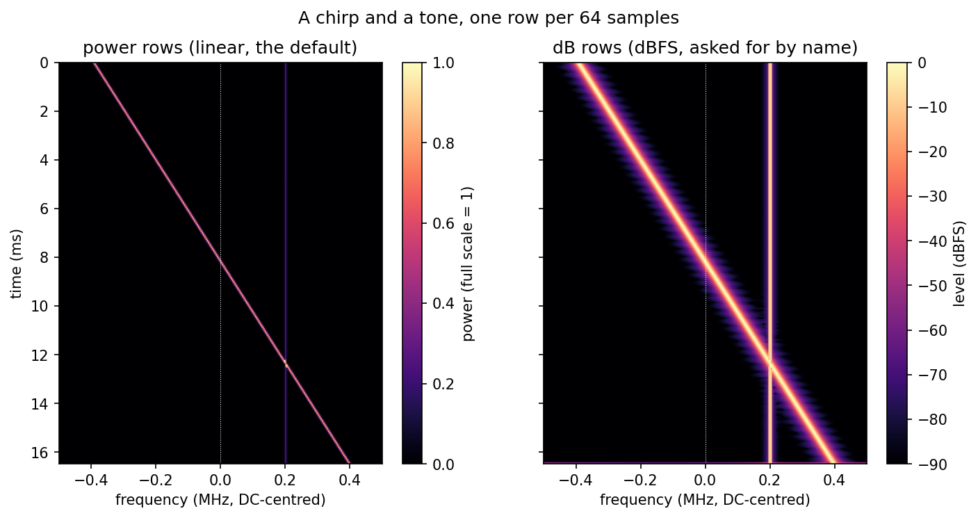
Both panels show the same capture: a complex chirp sweeping from −0.4 fs to +0.4 fs, and a tone at +0.2 fs at half amplitude. Each horizontal line is one row of the spectrogram: the power spectrum of one 256-sample frame, a new frame every 64 samples. Time runs down the page. The bottom row is the partial frame flushed at the end, zero-padded to a full frame, so its levels are lower and a little smeared.
The horizontal axis is DC-centred. Zero hertz is in the middle, and the edges are ±fs/2 = ±0.5 MHz. A frequency reads straight off the axis, with no shifting to do.
The left panel is power. A unit-amplitude tone reads 1.0 at its bin. The chirp is a bright diagonal line, because at any instant it sits on one bin at full scale. The tone is a dimmer vertical line: half the amplitude is a quarter of the power. Where the chirp crosses the tone, the two add coherently in that bin, so power there can read above 1.0, past the top of the colour bar.
The right panel is the same data in dBFS. Full scale is 0 dB, and the tone reads −6.02 dB, which is what the amplitude says it should. Each dB row is 10·log10 of the matching power row. Use dB when the levels span a wide range, and power when you want to add rows together: averaging dB rows gives a different answer from converting the average.
Power rows are the default. A dB spectrogram is asked for by name.
How it works
Samples arrive in pieces of any size, as they would from a radio, and the object turns them into rows as the frames complete. The example pushes the stream in random chunks, and the script checks that the rows match a single push of the whole capture. The chunk sizes do not change the rows. At the end the stream is flushed, which returns the zero-padded partial frame if one is owed:
def stream_rows(
    x: np.ndarray,
    mode: str,
    nfft: int,
    hop: int,
    chunked: bool = True,
) -> np.ndarray:
    """Return every row a stream produces, pushed in chunks or all at once."""
    sp = Spectrogram(nfft=nfft, hop=hop, window="hann", mode=mode)
    rows = []
    rng = np.random.default_rng(0)
    pos = 0
    while pos < x.size:
        size = int(rng.integers(1, 3 * nfft)) if chunked else x.size
        block = sp.push(x[pos : pos + size])
        if block is not None:  # None: this push completed no row
            rows.append(block)
        pos += size
    tail = sp.flush()  # a trailing partial frame, zero-padded, if one is owed
    if tail is not None:
        rows.append(tail)
    return np.concatenate(rows)
The figure is drawn from the rows the same stream produces. The checks in that function fail the run, not just the picture. They confirm that the chirp's peak stays within one bin of its sweep on every row, including the flushed partial row. They confirm the tone reads a quarter of full scale and −6.02 dB on every row the chirp is clear of, and that each dB row is 10·log10 of its power row. They also confirm the axis edges sit at ±0.5 MHz:
def make_figure(out_path: str = "spectrogram_demo.png") -> None:
    """Draw the chirp and tone as power and dB rows, after checking them."""
    n = np.arange(CAPTURE)
    t = n / FS
    total = CAPTURE / FS
    f0, f1 = -0.4 * FS, 0.4 * FS
    k = (f1 - f0) / total
    chirp = np.exp(2j * np.pi * (f0 * t + 0.5 * k * t * t))
    # On a bin centre, so the reading is the bin's own -6.02 dB.
    f_tone = 51 * FS / NFFT
    tone = 0.5 * np.exp(2j * np.pi * f_tone * t)
    x = (chirp + tone).astype(np.complex64)

    power = stream_rows(x, "power", NFFT, HOP)
    db = stream_rows(x, "db", NFFT, HOP)
    assert power.shape == db.shape
    # 254 whole frames, then the owed partial one, flushed at the end.
    assert power.shape[0] == 255
    # Chunking must not change the rows: compare with one push.
    assert np.array_equal(
        power, stream_rows(x, "power", NFFT, HOP, chunked=False)
    )

    bin_hz = FS / NFFT
    freqs = np.fft.fftshift(np.fft.fftfreq(NFFT, 1 / FS))
    # The bins span -fs/2 to +fs/2 exactly, so the axis edges are these.
    assert np.isclose(freqs[0], -FS / 2)
    assert np.isclose(freqs[-1] + bin_hz, FS / 2)

    rows = np.arange(power.shape[0])
    centre = (rows * HOP + NFFT / 2) / FS
    expect_hz = f0 + k * centre
    far = np.abs(expect_hz - f_tone) > 4 * bin_hz
    # The chirp's peak tracks the sweep within one bin, the flushed row too.
    peak_hz = (power.argmax(axis=1) - NFFT // 2) * bin_hz
    assert np.all(np.abs(peak_hz[far] - expect_hz[far]) <= bin_hz), np.abs(
        peak_hz[far] - expect_hz[far]
    ).max()
    tone_bin = NFFT // 2 + 51
    # The tone reads a quarter of full scale, and -6.02 dB, on every row clear
    # of the chirp.
    assert far.sum() > 200
    assert np.all(np.abs(power[far, tone_bin] - 0.25) < 0.02)
    assert np.all(np.abs(db[far, tone_bin] + 6.02) < 0.2)
    # Each dB row is 10 log10 of its power row, above the -90 dB floor.
    live = power > 1e-9
    assert np.allclose(db[live], 10 * np.log10(power[live]), atol=1e-3)

    fig, (ax_p, ax_d) = plt.subplots(1, 2, figsize=(11, 5), sharey=True)
    # MHz across; ms down, with row 0 (time 0) at the top of the panel.
    extent = (freqs[0] / 1e6, (freqs[-1] + bin_hz) / 1e6, total * 1e3, 0.0)
    im_p = ax_p.imshow(
        power,
        origin="upper",
        aspect="auto",
        extent=extent,
        vmin=0.0,
        vmax=1.0,
        cmap="magma",
    )
    im_d = ax_d.imshow(
        db,
        origin="upper",
        aspect="auto",
        extent=extent,
        vmin=-90.0,
        vmax=0.0,
        cmap="magma",
    )
    ax_p.set_title("power rows (linear, the default)")
    ax_d.set_title("dB rows (dBFS, asked for by name)")
    for ax in (ax_p, ax_d):
        ax.set_xlabel("frequency (MHz, DC-centred)")
        ax.axvline(0.0, color="w", lw=0.5, ls=":")
    ax_p.set_ylabel("time (ms)")
    fig.colorbar(im_p, ax=ax_p, label="power (full scale = 1)")
    fig.colorbar(im_d, ax=ax_d, label="level (dBFS)")
    fig.suptitle("A chirp and a tone, one row per 64 samples")
    fig.savefig(out_path, dpi=150, bbox_inches="tight")
    plt.close(fig)
Running it
The script writes spectrogram_scene.png and spectrogram_demo.png in the
working directory, and exits
0 only when its checks hold.