DSSS Acquisition — Pd / Pfa vs Es/N0
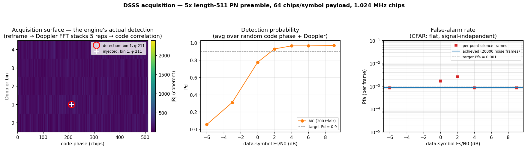
A performance characterisation of doppler.acquire.BurstAcquisition on a DSSS preamble: the probability
of detection (Pd) and probability of false alarm (Pfa) of a
spread-spectrum burst acquirer, measured by Monte-Carlo against the data-link
Es/N0.
The scenario
A direct-sequence transmitter emits a burst:
- Acquisition preamble — a 9-stage Galois maximum-length sequence (period
2⁹ − 1 = 511chips), repeated 5 times so the receiver can integrate it coherently. - Payload — random BPSK data spread at 64 chips per symbol over a distinct code, so it decorrelates from the preamble.
- Channel — the burst arrives at a random integer code phase and a
random carrier (Doppler) offset, uniform across the engine's
±
chip_rate/(2·sf)≈ ±1 kHz capture range, buried in AWGN. Chip rate is 1.024 MHz.
Everything radiated is built through the wfm wfmgen surface —
Synth(type="pn") for the preamble, dsss_spread for the payload. Only the
channel (delay, Doppler, silence, AWGN) is applied around it.
What you're seeing
Left — the acquisition surface and the actual detection. This is the
engine's own decision surface for the preamble frame, reconstructed exactly as
it computes it: reframe the frame into (5, 511) (one row per code
repetition), take the slow-time Doppler FFT down the rows — which
coherently stacks all five repetitions for the full 10·log10(5·511) ≈ 34
dB gain — then circularly correlate each row against the PN code. The single
bright cell is the peak; the red circle is the engine's actual emitted
detection and the white cross is the injected cell. Here both sit at
(Doppler bin 1, code phase 211) — the engine acquired the right
(Doppler, delay) index, and the surface is flat noise everywhere else (the
PN code's near-ideal autocorrelation). This coherent stack is why the burst
is detectable even though the raw signal sits below the noise — the defining
DSSS property.
Centre — Pd vs Es/N0. The Monte-Carlo S-curve, averaged over random code
phase and random Doppler across the capture range, passing through the
configured pd = 0.9 target. The knee sits a few dB above the raw
10·log10(sf·reps) ≈ 34 dB coherent gain because the average folds in the
Doppler scalloping and within-segment rotation losses of the coarse 5-bin
search — an honest operating curve, not the on-bin best case.
Right — Pfa vs Es/N0. The false-alarm rate, measured on the noise-only
(silence) frames. It is set by the engine's CFAR threshold and is independent
of the signal, so it stays flat across the whole sweep, at or just under
the configured pfa = 1e-3. The solid line is the achieved rate over a
20 000-frame noise-only run: 8.5e-4, 0.85× the target (−0.7 sigma). The
gate is priced over every row of the Doppler-interpolated surface its
maximum ranges over, a never-exceed bound
(#2218; the measured
refinement is #1064).
Priced over the native rows, it fired at 1.85×. This run holds the ratio under
1.4×, a loose check at 20 000 frames (an on-target detector exceeds it by
chance about 3% of the time); the certification holds the same bound over
60 000. The squares are the noisier
per-Es/N0 estimates.
How it works
BurstAcquisition is constructed from physics, not tuning knobs — the
preamble's samples (the PN code by bin_to_nrz, each chip held spc samples),
their rate fs = chip_rate·spc, the repetitions reps, a sizing sensitivity
(cn0_dbhz), and the detection targets (pfa, pd). It then:
- Frames the raw stream into
(doppler_bins, code_bins)wherecode_bins = sf·spcis one PN segment (the fast-time / code-phase axis) anddoppler_binsis the coherent depth (≤reps). - Runs a slow-time Doppler FFT along the segment axis.
- Correlates against the single-row PN reference (the circular code matched filter on the fast-time axis).
- Estimates a CFAR noise floor and gates the peak — emitting an
(doppler_bin, code_phase, …)event whenever the test statistic crosses an automatically configured, Bonferroni-corrected threshold.
The script pins the coherent depth to all five repetitions with
configure_search_raw(reps, 1) (doppler_bins == reps), so one acquisition
frame spans the whole preamble.
Es/N0
With a unit-power chip and complex AWGN of per-sample variance σ² (per-sample
power SNR γ = 1/σ²):
Ec/N0 = spc · γ                       per chip      (+10·log10(spc) dB)
Es/N0 = DATA_SF · Ec/N0               per data symbol (DATA_SF chips)
      → Es/N0_dB = snr_db + 10·log10(DATA_SF · spc)
At spc = 1 that is a flat +10·log10(64) = +18.06 dB offset from the
per-sample SNR the engine sizes against — the x-axis of the two operating
curves.
Run it
This is a characterization, not an example: it sweeps a noise floor over many trials, so it is run deliberately rather than on every push. See Object Validation for the distinction.
make characterize          # every subject

python -m \
    doppler.acquire.tests.characterization.burst_acquisition.characterize
The waveform geometry, signal construction, and the (Doppler bin, code phase)
mapping live in
doppler.acquire.tests.characterization.burst_acquisition.characterize, shared
with the test_acq_characterization gate so the sweep and the test agree by
construction.