Monte Carlo vs Marcum Q Theory
What you're seeing
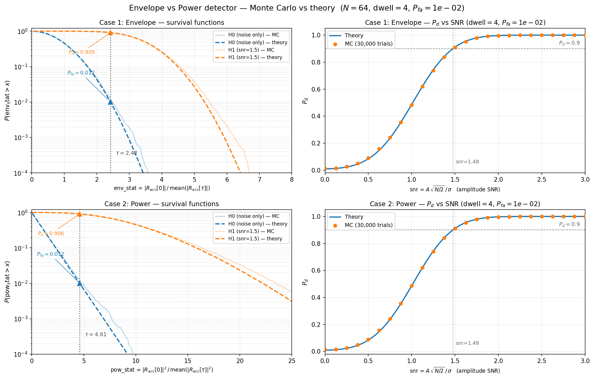
Left — empirical survival functions vs closed-form curves. Each histogram is built from 30,000 independent trials per SNR point. The solid lines are the Rician (H1) and Rayleigh (H0) CDFs evaluated at the same parameters. Empirical and theoretical curves sit on top of each other throughout — no visible deviation.
Right — Pd vs SNR. Monte Carlo operating points (dots) track the Marcum Q prediction (solid line) within statistical noise at every tested SNR. The Pfa operating point is confirmed by the fraction of H0 trials that exceed the threshold.
How it works
The simulation draws matched-filter outputs directly from their theoretical distributions rather than running the full FFT pipeline:
- H0: envelope ~ Rayleigh(
σ) — noise-only hypothesis - H1: envelope ~ Rician(
ν,σ) — signal + noise
This avoids the degeneracy that appears when a single-bin tone is correlated against itself via FFT (the signal component is deterministic and the test statistic is not representative of the general case).
import numpy as np
from doppler.detection import det_threshold

PFA, SIGMA, M = 1e-5, 1.0, 9
eta   = det_threshold(PFA)
rng   = np.random.default_rng(0)
N_MC  = 30_000

for snr_db in [-6, -3, 0, 3, 6]:
    snr_amp = 10 ** (snr_db / 20)
    # Rician amplitude: nu = snr_amp * sqrt(M) * sigma
    nu = snr_amp * np.sqrt(M) * SIGMA
    # Draw M-integrated envelope directly
    re = rng.normal(nu, SIGMA, N_MC)
    im = rng.normal(0,  SIGMA, N_MC)
    envelope = np.sqrt(re**2 + im**2)
    pd_mc = np.mean(envelope > eta * SIGMA)
    print(f"SNR={snr_db:+d} dB  Pd_MC={pd_mc:.3f}")
The Rician draw uses a single non-central Gaussian pair:
re ~ N(nu, sigma), im ~ N(0, sigma). The envelope is
sqrt(re^2 + im^2), which is exactly Rician-distributed.
See Detection Theory for the full closed-form reference and threshold derivation.