M-PSK Receiver — Sizing the Carrier Loop, and Riding a Doppler Profile
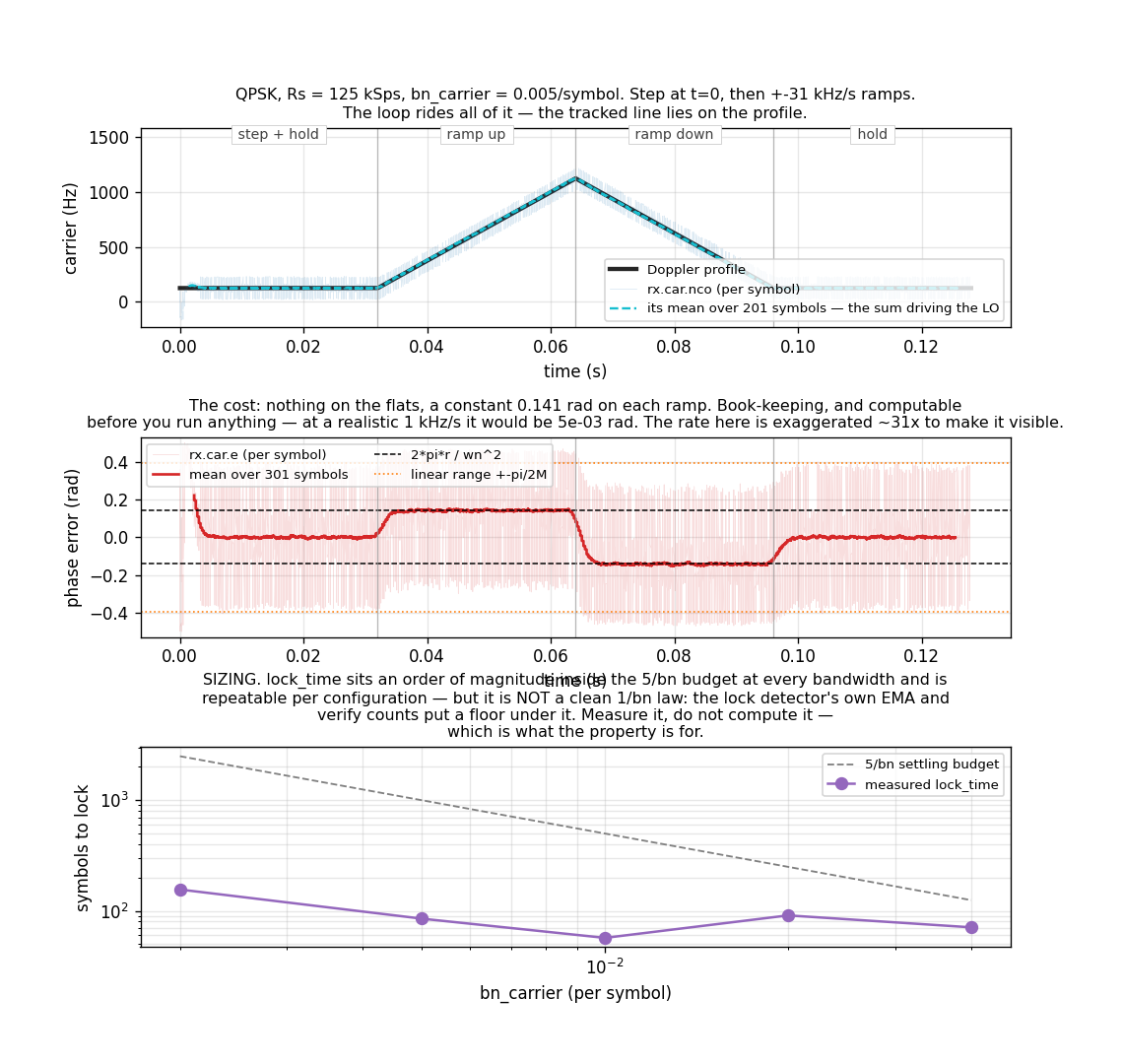
A track.MpskReceiver is handed a carrier that steps,
then ramps up, then ramps down, then holds. It rides all of it.
The practical question is not whether it copes — it does — but how to size
bn_carrier so acquisition happens in a time you can plan around, and what
the profile costs once it has. The short answers: a step is free, a ramp is
very cheap, and acquisition time is something to measure, not compute.
A step is free; a ramp is very cheap
The carrier loop filter is type 2 — a PI filter feeding a phase accumulator. Against a frequency step its steady-state phase error is zero regardless of loop gain. Against a ramp it holds a constant phase offset:
with \(r\) the Doppler rate in cycles/symbol². That is the middle panel, and the measured mean lands within 1% of the closed form on both ramps.
It is book-keeping. At the figure's settings the offset is 0.141 rad, but that rate is exaggerated ~31× to make it visible at all: at a realistic 1 kHz/s the same formula gives 4.5e-3 rad, roughly 1% of the discriminator's \(\pi/2M\) linear range. It costs no decisions. You can compute it before you run anything, and usually then ignore it.
The offset only matters when it approaches that linear range — which is the
real Doppler-rate ceiling of a given bn_carrier, and since \(\theta_{ss}\) goes
as \(1/\omega_n^2\), the maximum trackable rate goes as \(b_n^2\).
Sizing: measure the acquisition time, do not compute it
The bottom panel is the decision that actually matters. Acquisition sits an
order of magnitude inside the classical 5/bn settling budget at every
bandwidth, and is repeatable per configuration — the seed-to-seed spread is
a few percent.
But it is not a clean 1/bn law, and the page says so because the tidy
version is tempting and wrong. Measured across five seeds, bn = 0.01 comes
out bimodal (140/140/139/57/57) and the trend is not monotonic. The lock
detector has its own dynamics — an EMA at CARRIER_NDA_LOCK_ALPHA = 0.05 and a
verify count in each direction — which puts a floor under the loop's settling
and makes declaration a threshold crossing rather than a settling time.
So: pick bn_carrier from the loop bandwidth your link needs, then read
lock_time back for your configuration. That is what
the property exists for.
rx = MpskReceiver(m=4, sps=8, m_out=4, bn_carrier=0.005)
rx.steps(iq)
rx.lock_time  # symbols to the FIRST lock declaration, or -1 if never
The top panel plots the sum, not the integrator
rx.car.nco is the command that actually drives the LO: integ + kp*e.
rx.car.freq is the integrator alone — the frequency memory, which is
what survives a handover — and on a ramp the two differ by exactly the
proportional term. Measured on the ramp up: the sum lags by 4.4e-06
cycles/sample against a 1.0e-03 excursion, the integrator by 3.3e-05, a factor
of 7.5.
Publishing only the integrator made a correctly-tracking loop look like it was lagging, which is why the sum is now a probe in its own right.
Its per-symbol variance is large — that is the light band in the top panel —
because the proportional term carries the discriminator's full data noise. Its
mean is what tracks the ramp, exactly as get_nco_freq() documents.
Why measure ramps at all, if they are cheap
Because a step-only test cannot size a loop. A type-2 loop nulls a step
whatever its gain, so a loop running several times narrower than configured
passes every step test unchanged. That is not hypothetical: it is how
freq_scale under-drove every non-strobe NDA tap in this library until a
ramp measurement found it
(gh-765).
native/validation/rx_dynamics.c now gates the closed form.
Telemetry, not reconstruction
Every trace is a probe the receiver already publishes, captured losslessly at
decim=1 through Telemetry and a
MemoryCapture. Nothing here re-derives a loop internal from the output
symbols.
import numpy as np

from doppler.telemetry import MemoryCapture, Telemetry
from doppler.track import MpskReceiver
from doppler.wfm import SampleClock

FS = 1e6  # sample rate (Hz) — the figure's time axis
SPS = 8  # samples/symbol -> Rs = 125 kSps
M = 4  # QPSK
BN = 0.005  # carrier loop noise bandwidth, per SYMBOL
NSEG = 4000  # symbols per profile segment (4x the 5/bn settling)
BLOCK = 256

# The Doppler profile, in cycles/sample. A STEP the cold-started loop has to
# find, then a ramp UP, then a ramp DOWN of the same rate — so the frequency
# comes back to where it started — then flat.
# The step has to be one a COLD loop can actually find: an M-th-power NDA
# loop pulls in |df| up to about bn/M per symbol, which is 0.00125 here, and
# pull-in time grows as df^2/bn^3 past it. 0.001 cycles/symbol is 0.8 of that
# bound — a real acquisition, not a seeded one.
F0_SYM = 0.001  # cycles/SYMBOL
F0 = F0_SYM / SPS  # cycles/sample
RATE_SYM = 2.0e-6  # Doppler RATE, cycles/symbol^2
a = RATE_SYM / SPS**2  # the same rate per sample^2

nseg = NSEG * SPS
seg = np.arange(nseg)
freq = np.concatenate(
    [
        np.full(nseg, F0),  # A: step, then hold
        F0 + a * seg,  # B: ramp up
        F0 + a * nseg - a * seg,  # C: ramp down
        np.full(nseg, F0),  # D: hold again
    ]
)

# Phase is the running sum of frequency — the discrete-time NCO's own
# definition, so the segment joins carry no phase discontinuity to explain.
rng = np.random.default_rng(7)
idx = rng.integers(0, M, freq.size // SPS)
tx = np.exp(1j * (2 * np.pi * idx / M + np.pi / M)).astype(np.complex64)
tx = np.repeat(tx, SPS)
ph = 2.0 * np.pi * np.cumsum(freq)
iq = (tx * np.exp(1j * ph)).astype(np.complex64)

# `strobe` is the default tap: it reads the on-time strobe, at the full
# post-matched-filter SNR. Nothing here depends on that choice — the loop
# stress below is a property of bn_carrier, not of where the detector reads.
rx = MpskReceiver(m=M, sps=SPS, m_out=4, bn_carrier=BN, bn_timing=0.005)

tlm = Telemetry()
rx.set_telemetry(tlm, "rx", 1)  # decim=1: every probe, every symbol
with MemoryCapture(tlm, BLOCK, SampleClock(FS)) as cap:
    for i in range(0, iq.size, BLOCK):
        tlm.set_now(i)
        rx.steps(iq[i : i + BLOCK])
series = cap.read_dict(index=True)  # {name: (sample_index, values)}

n_e, err = series["rx.car.e"]  # phase error (book-keeping, see below)
n_f, fhat = series["rx.car.nco"]  # the SUM that drives the LO: integ + kp*e
n_i, fint = series["rx.car.freq"]  # the integrator alone — the freq MEMORY
n_l, lock = series["rx.lock"]

# Sizing: acquisition time against bn. The same ASK at every bandwidth (a
# step at 0.8 of the bn/M seeding bound), so the only thing varying is the
# loop. This is the middle panel and the practical result.
BN_GRID = (0.002, 0.005, 0.01, 0.02, 0.04)


def acquire_in(bn: float, nsym: int = 20000) -> int:
    """Symbols to first lock declaration at loop bandwidth `bn`."""
    r2 = np.random.default_rng(3)
    i2 = r2.integers(0, M, nsym)
    t2 = np.exp(1j * (2 * np.pi * i2 / M + np.pi / M)).astype(np.complex64)
    t2 = np.repeat(t2, SPS)
    k2 = np.arange(t2.size)
    f_step = 0.8 * bn / M / SPS  # 0.8 of the seeding bound, in cyc/sample
    x2 = (t2 * np.exp(2j * np.pi * f_step * k2)).astype(np.complex64)
    r = MpskReceiver(m=M, sps=SPS, m_out=4, bn_carrier=bn, bn_timing=0.005)
    r.steps(x2)
    return int(r.lock_time)


lock_times = [acquire_in(b) for b in BN_GRID]

# The closed form this figure exists to show, in the loop's own units.
wn = 8.0 * 0.707 * BN / (4.0 * 0.707**2 + 1.0)  # rad/symbol
theta_ss = 2.0 * np.pi * RATE_SYM / wn**2  # rad
linear_range = np.pi / (2 * M)  # M-th power S-curve
The step has to be one a cold loop can find
F0_SYM is 0.001 cycles/symbol, which is 0.8 of the bn/M seeding bound. Past
that bound an M-th-power NDA loop still acquires, but pull-in time grows as
\(\Delta f^2/b_n^3\) — the first draft of this example used a step 6.4× the bound
and the receiver had not locked by the end of a 16 000-symbol record. If a cold
acquisition is taking implausibly long, that ratio is the first thing to check.
Related pages
- M-PSK Receiver — the constellation, lock and BER story.
- M-PSK Receiver: Performance — EVM, SER and lock time over random geometries.
- Design note — the two-clock architecture, the NDA taps, and where the discriminator reads.