M-PSK Receiver — Performance Characterisation¶

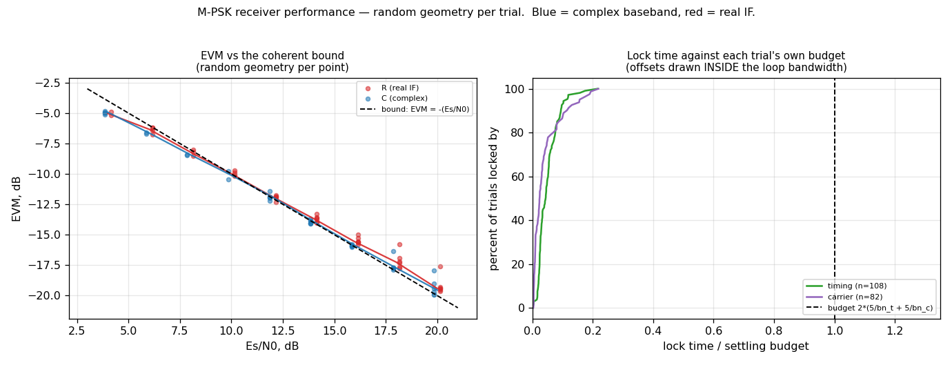
This is the receiver's characterisation, not a demo of it. Everything on the page is measured over randomly drawn geometries rather than a fixed grid, on both track.MpskReceiver (complex baseband) and track.MpskReceiverR (real IF) — see the walkthrough page for what they are and the design note for how they work.

Each trial independently draws the constellation order, m_out, a non-integer samples-per-symbol, the IF placement, both loop bandwidths, the frequency and clock offsets, the absolute level, and the data. That is the point:

Why random draws, not a grid

A grid measures the geometries you thought of. Random draws over the documented input domain either show you a clean distribution or hand you the outlier — and that is exactly how a real one hid here for weeks: at sps = 10 with m_out = 4 and an IF at 0.10, the occupied band reaches DC, where the real front end's image rejection collapses. No grid of "reasonable" cases drew it.

That case has since been traced and fixed — the R2C halfband returned half the amplitude the analytic-signal convention requires, so the real path ran 6 dB down and the timing loop 4× under-driven, and the −4 dB was the under-drive rather than the placement. It now measures −20 dB with zero SER, and the placement tolerance is documented as the geometric rule it always was (1/sps < fc < 0.5 − 1/sps; see the design note). The draw is what found it, and that is the part worth keeping.

The measurement rules the panels obey¶

These are not incidental — get any of them wrong and the numbers look like DSP defects. They are the same rules the design note and the receiver's test harness encode.

Rule	Why
Settling = `2·(5/bn_t + 5/bn_c)`	5/Bn per loop; the two add because they are cascaded (the carrier discriminator reads the on-time strobe, so it cannot converge until timing has); then double for joint tracking, where each loop sees the other's transient. Measuring from `5/bn` alone reads −9.0 dB where the settled answer is −23.2 dB.
Offsets INSIDE the loop bandwidth	Seeded on truth, the loop never leaves its initial state and any lock time is meaningless. Asserted outside `Bn`, the test measures luck. Measured: carrier lock in 39 symbols at `0.25·Bn`, 1376 at `1·Bn`, never at `2·Bn`.
Loop SNR ≈ 20 dB, `bn ≤ 0.01`	`ρ_L = Es/N0 + squaring_loss − 10log₁₀(bn)`. Below ~20 dB the loop is driven by noise: the estimate random-walks and the receiver declares lock while producing chance-level symbols. If you are short of it, narrow `bn` — never accept less.
Never widen `bn` for a shorter record	`bn` is normalised to the symbol rate, so settling is a fixed number of symbols at any sample rate. Widening does not buy samples, it changes the receiver. A heavily oversampled case simply needs millions of samples — that is what `wfmgen` is for.
Anchor at SER = 1e-3	Per-M that is 6.8 / 10.3 / 15.7 dB, which asks "does it meet its bound" at the same place on the curve for every order, instead of at one arbitrary Es/N0.

The two panels¶

EVM vs the coherent bound. Self-referenced EVM — each symbol against its own hard decision — against EVM_dB = −(Es/N0)_dB. EVM is an I/Q-plane quantity, so there is no factor of two, and an EVM beating the bound means the measurement is wrong. Median margin over the whole random sweep: +0.2 dB.

Some trials carry no measurement, and the demo says so

A trial whose timing rate is still slewing at the end of its record has no window in which one detected alignment is valid — the receiver is emitting at slightly the wrong cadence, so the rx-to-truth lag moves inside the window. BerMeter scores a detected lag verbatim, so such a window reads correct at its start and chance after it: measured, lag 18 becoming 19, and an SER of 0.483 on a receiver whose settled SER over the same capture is 0.

That is not a lock failure and must not be scored as one. Those trials are refused and counted in the output rather than dropped, because a refusal nobody counts is indistinguishable from a measurement nobody made. The underlying cause — 5/Bn is a phase-settling budget and does not cover slewing out a clock offset, measured 12.7× short — is doppler#1060.

Lock time against each trial's own budget. Not an absolute symbol count — a fraction of that trial's 2·(5/bn_t + 5/bn_c), which is the only way to compare trials with different loop bandwidths.

Six more panels exist, on demand

--only ber,falsealarm,level,invariance,chunking,telemetry, or --only all. They are not in the committed figure because each answers a PASS/FAIL question, and a plot is the wrong shape for one: level and sample-rate invariance are flat lines, false alarm is a count of zero, chunking is a bar chart of exact zeros, telemetry is two bars, and ber restates evm on a log axis.

All six are assertions instead, which is where a pass/fail property belongs — it then runs on every commit rather than sitting in a PNG: src/doppler/track/tests/test_mpsk_receiver_performance.py covers false alarm, level invariance and the coherent bound, and the bench_mpsk_receiver*.py pair covers the telemetry cost (+10.5% complex, +11.6% real).

How the SER is measured, since it is easy to get wrong

The bound test stops on a fixed number of errors, not symbols. Under inverse binomial sampling the symbol count is the random variable (negative-binomially distributed) and the relative standard error is 1/√r — dependent only on the error count, so the target error count is the precision. 200 errors gives ~7% relative, ±14% at 95%. A fixed 20 000-symbol burst at SER 1e-3 yields ~20 errors and ~22% relative error, which reads as real seed-to-seed variation in the receiver.

Two consequences a fixed-N measurement misses: the naive r/N is biased (the unbiased estimator is (r−1)/(N−1)), and the interval comes from the negative binomial rather than a binomial on a fixed N.

Also compare like with like: a differential SER is rotation-free, and therefore convenient, but a differential decision fails if either of its two symbols is wrong — so it reads ~2× a coherent SER (measured 1.88–2.11 here). Comparing one against a coherent curve invents a factor of two of "implementation loss". Measured coherently, both receivers sit 1.2–2.4× the bound, i.e. 0.3–1.0 dB, with 8PSK on the real IF the only cell above 2×.

A rotation-blind metric cannot check your measurement window

Self-referenced EVM and the hard-decision phase error both estimate the constellation rotation from the data, so a constellation that is still rotating reads clean on both while decoding to the wrong symbols. Measured on 8PSK: EVM within 0.3 dB of the bound, phase-error mean −0.0002 rad, and not one symbol beyond the ±π/8 decision boundary — beside an SER six times the bound. Two independent truth-free validators agreed with each other and both were blind to it.

The cause was the window, and specifically the handover the receiver carried at the time: with acq_to_track enabled it fired on carrier lock plus a warmup, later than the analytic 5/Bn budget and later than every lock indicator, and the decision-directed loop then had its own transient. It landed at symbol 2525 against a 2000-symbol budget; measuring from 2000 read 5.95× the bound where the settled answer is 1.68×. The handover is gone (#877) and this particular trap with it, but the lesson is not about handovers: localise a suspected window fault by asking where the errors are — an error rate per block across the record — not by adding another truth-free metric.

Streaming a real capture in¶

The receivers are streaming objects: state carries across calls, so a capture arrives in whatever blocks your transport hands you.

# Feeding a stream in chunks: the receiver is a streaming object, so `steps()`
# may be called with whatever block the source hands you. It keeps every piece
# of state that spans a call -- the LO phase, the cascade's delay lines, the
# timing accumulator, both loop integrators, and (on the real path) the R2C
# halfband's orphan sample when a chunk has odd length -- so a chunked run is
# BIT-IDENTICAL to one big call. Chunk size is a buffering decision, not a
# signal-processing one.
import numpy as np  # noqa: E402  (region must be self-contained)


def demod_stream(rx, blocks):
    """Feed an iterable of blocks; yield the symbols each call produced.

    The output count per call VARIES -- a chunk of N samples yields about
    N/sps symbols, but which side of the boundary a symbol lands on depends
    on the timing accumulator's phase, so never assume a fixed ratio.
    """
    for block in blocks:
        symbols = rx.steps(block)  # may be empty for a short block
        if len(symbols):
            yield symbols


def chunk_randomly(x, rng, lo=997, hi=9973):
    """Split `x` into chunks of random length -- deliberately including ODD
    lengths, which is what exercises the real path's even/odd halfband pairing
    across a call boundary."""
    i = 0
    while i < x.size:
        n = int(rng.integers(lo, hi))
        yield x[i : i + n]
        i += n

Reproduce¶

Every panel is independently selectable, so a single question is cheap to ask:

# the two panels above (the default, and what the figure is)
python src/doppler/examples/mpsk_receiver_performance_demo.py

# every panel, including the six pass/fail ones
python src/doppler/examples/mpsk_receiver_performance_demo.py --only all

# one question at a time
python src/doppler/examples/mpsk_receiver_performance_demo.py --only falsealarm

# more draws for a tighter distribution
python src/doppler/examples/mpsk_receiver_performance_demo.py --trials 400

Not run by the examples gate

This script is listed in src/doppler/examples/.examples-skip. Its Monte Carlo asserts the coherent bound, and 8PSK at m_out < 8 genuinely misses it (measured 8.1 dB of loss at m_out = 4, sps = 10.73), so pass/fail depends on the draw. Everything it measures about the shipped defaults is covered by src/doppler/track/tests/, which does run in CI.